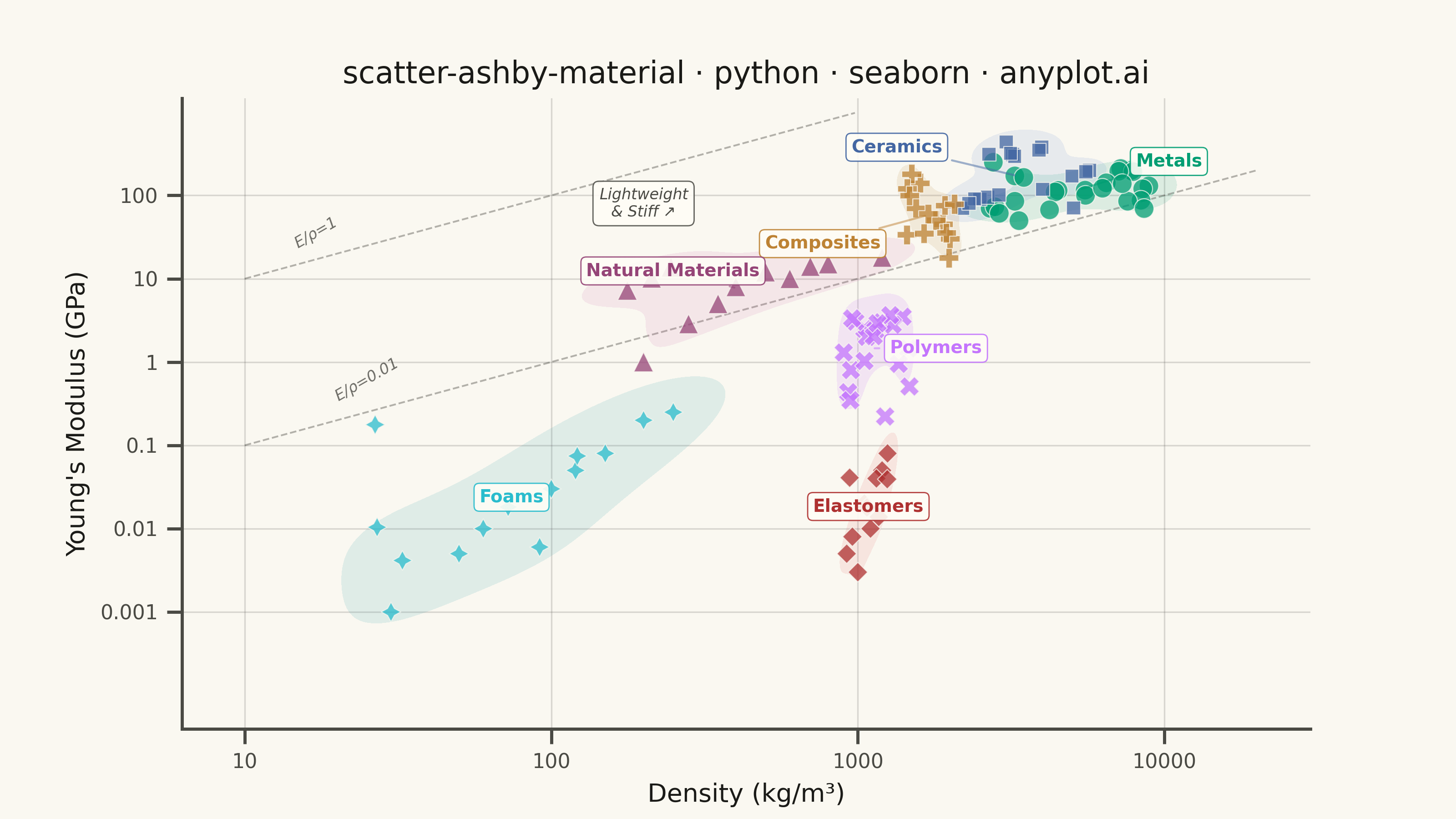
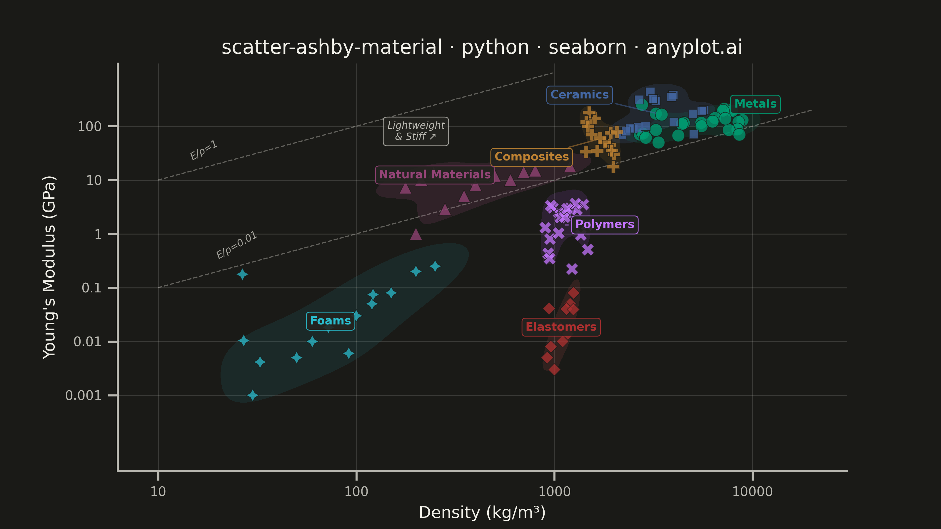
A log-log scatter plot comparing two material properties (e.g., Young's modulus vs. density) with material families displayed as labeled bubble regions. Developed by Michael Ashby for systematic material selection in engineering design, this chart enables rapid visual comparison of material classes across multiple property dimensions. It is a standard tool in materials science and mechanical engineering education.
""" anyplot.ai
scatter-ashby-material: Ashby Material Selection Chart
Library: seaborn 0.13.2 | Python 3.13.13
Quality: 91/100 | Updated: 2026-06-03
"""

import os
import sys


# Remove the script's own directory from sys.path so that matplotlib.py (a sibling
# implementation file) does not shadow the installed matplotlib package.
_this_dir = os.path.dirname(os.path.abspath(__file__))
sys.path = [p for p in sys.path if os.path.abspath(p or ".") != _this_dir]

import matplotlib.pyplot as plt
import numpy as np
import pandas as pd
import seaborn as sns


# Theme tokens (see prompts/default-style-guide.md "Theme-adaptive Chrome")
THEME = os.getenv("ANYPLOT_THEME", "light")
PAGE_BG = "#FAF8F1" if THEME == "light" else "#1A1A17"
ELEVATED_BG = "#FFFDF6" if THEME == "light" else "#242420"
INK = "#1A1A17" if THEME == "light" else "#F0EFE8"
INK_SOFT = "#4A4A44" if THEME == "light" else "#B8B7B0"
INK_MUTED = "#6B6A63" if THEME == "light" else "#A8A79F"

# Imprint palette — canonical order, 7 positions for 7 material families
IMPRINT_PALETTE = ["#009E73", "#C475FD", "#4467A3", "#BD8233", "#AE3030", "#2ABCCD", "#954477"]

sns.set_theme(
    style="ticks",
    rc={
        "figure.facecolor": PAGE_BG,
        "axes.facecolor": PAGE_BG,
        "axes.edgecolor": INK_SOFT,
        "axes.labelcolor": INK,
        "text.color": INK,
        "xtick.color": INK_SOFT,
        "ytick.color": INK_SOFT,
        "grid.color": INK,
        "grid.alpha": 0.15,
        "legend.facecolor": ELEVATED_BG,
        "legend.edgecolor": INK_SOFT,
    },
)

# Data — density (kg/m³) vs Young's modulus (GPa) for common engineering materials
np.random.seed(42)

families = {
    "Metals": {
        "density": (2700, 8900),
        "modulus": (45, 400),
        "n": 25,
        "materials": [
            (2700, 70),
            (4500, 115),
            (7800, 200),
            (7200, 210),
            (8900, 130),
            (8500, 120),
            (7900, 193),
            (4400, 110),
            (2800, 73),
            (7100, 195),
        ],
    },
    "Polymers": {
        "density": (900, 1500),
        "modulus": (0.2, 4.0),
        "n": 20,
        "materials": [
            (950, 0.8),
            (1050, 2.5),
            (1200, 3.0),
            (1400, 3.5),
            (1140, 2.4),
            (900, 1.3),
            (1300, 2.8),
            (1070, 2.0),
        ],
    },
    "Ceramics": {
        "density": (2200, 6000),
        "modulus": (70, 450),
        "n": 18,
        "materials": [
            (3980, 380),
            (2200, 70),
            (3200, 310),
            (5700, 200),
            (2500, 90),
            (3900, 350),
            (5000, 170),
            (2650, 95),
        ],
    },
    "Composites": {
        "density": (1400, 2200),
        "modulus": (15, 200),
        "n": 15,
        "materials": [
            (1600, 140),
            (1900, 45),
            (1500, 180),
            (2000, 30),
            (1550, 70),
            (1800, 50),
            (1450, 120),
            (1700, 60),
        ],
    },
    "Elastomers": {
        "density": (900, 1300),
        "modulus": (0.002, 0.1),
        "n": 12,
        "materials": [
            (920, 0.005),
            (1100, 0.01),
            (1200, 0.05),
            (1000, 0.003),
            (1050, 0.02),
            (960, 0.008),
            (1150, 0.04),
            (1250, 0.08),
        ],
    },
    "Foams": {
        "density": (25, 300),
        "modulus": (0.001, 0.3),
        "n": 14,
        "materials": [
            (30, 0.001),
            (60, 0.01),
            (120, 0.05),
            (200, 0.2),
            (50, 0.005),
            (100, 0.03),
            (250, 0.25),
            (150, 0.08),
        ],
    },
    "Natural Materials": {
        "density": (150, 1300),
        "modulus": (0.1, 20),
        "n": 12,
        "materials": [(500, 12), (700, 14), (400, 8), (200, 1.0), (600, 10), (1200, 18), (350, 5), (800, 15)],
    },
}

rows = []
for family, props in families.items():
    for d, m in props["materials"]:
        rows.append({"family": family, "density": d, "modulus": m})
    extra_n = props["n"] - len(props["materials"])
    if extra_n > 0:
        log_d_min, log_d_max = np.log10(props["density"][0]), np.log10(props["density"][1])
        log_m_min, log_m_max = np.log10(props["modulus"][0]), np.log10(props["modulus"][1])
        extra_d = 10 ** np.random.uniform(log_d_min, log_d_max, extra_n)
        extra_m = 10 ** np.random.uniform(log_m_min, log_m_max, extra_n)
        for d, m in zip(extra_d, extra_m, strict=True):
            rows.append({"family": family, "density": d, "modulus": m})

df = pd.DataFrame(rows)
df["log_density"] = np.log10(df["density"])
df["log_modulus"] = np.log10(df["modulus"])

family_order = list(families.keys())
palette = dict(zip(family_order, IMPRINT_PALETTE, strict=False))

# Canvas — landscape 3200×1800 px (figsize=(8, 4.5) × dpi=400, no bbox_inches="tight")
fig, ax = plt.subplots(figsize=(8, 4.5), dpi=400, facecolor=PAGE_BG)
ax.set_facecolor(PAGE_BG)

# KDE envelopes — seaborn's idiomatic family-region feature (operates in log-space)
sns.kdeplot(
    data=df,
    x="log_density",
    y="log_modulus",
    hue="family",
    hue_order=family_order,
    palette=palette,
    levels=2,
    thresh=0.3,
    fill=True,
    alpha=0.12,
    linewidths=0,
    ax=ax,
    legend=False,
    zorder=1,
    common_norm=False,
)

# Scatter points
sns.scatterplot(
    data=df,
    x="log_density",
    y="log_modulus",
    hue="family",
    hue_order=family_order,
    palette=palette,
    style="family",
    s=60,
    alpha=0.75,
    edgecolor=PAGE_BG,
    linewidth=0.4,
    ax=ax,
    legend=False,
    zorder=3,
)

# Performance index guide lines E/ρ = const — ratios 0.01, 1, 100 (Ashby chart signature)
log_d_range = np.linspace(np.log10(10), np.log10(20000), 200)
guide_indices = [(0.01, "E/ρ=0.01"), (1.0, "E/ρ=1"), (100.0, "E/ρ=100")]
for ratio, label in guide_indices:
    log_m_line = np.log10(ratio) + log_d_range
    mask = (log_m_line >= np.log10(5e-4)) & (log_m_line <= np.log10(1000))
    if mask.sum() > 0:
        ax.plot(
            log_d_range[mask], log_m_line[mask], color=INK_MUTED, linewidth=0.7, linestyle="--", alpha=0.5, zorder=0
        )
        vis_d = log_d_range[mask]
        vis_m = log_m_line[mask]
        if len(vis_d) > 10:
            idx = int(len(vis_d) * 0.12)
            ax.text(
                vis_d[idx],
                vis_m[idx] + 0.1,
                label,
                fontsize=6,
                color=INK_MUTED,
                fontstyle="italic",
                rotation=30,
                ha="center",
                va="bottom",
                zorder=0,
            )

# Lightweight & stiff directional annotation
ax.annotate(
    "Lightweight\n& Stiff ↗",
    xy=(np.log10(200), np.log10(80)),
    fontsize=6,
    fontstyle="italic",
    color=INK_SOFT,
    ha="center",
    va="center",
    zorder=4,
    bbox={
        "boxstyle": "round,pad=0.4",
        "facecolor": ELEVATED_BG,
        "alpha": 0.85,
        "edgecolor": INK_SOFT,
        "linewidth": 0.5,
    },
)

# Family labels near cluster centroids
label_offsets = {
    "Metals": (0.3, 0.35),
    "Ceramics": (-0.4, 0.35),
    "Composites": (-0.35, -0.35),
    "Polymers": (0.2, 0.0),
    "Elastomers": (0.0, 0.0),
    "Foams": (0.0, 0.0),
    "Natural Materials": (-0.2, 0.2),
}

for family in family_order:
    subset = df[df["family"] == family]
    color = palette[family]
    centroid_log_d = subset["log_density"].mean()
    centroid_log_m = subset["log_modulus"].mean()
    offset = label_offsets.get(family, (0, 0))
    label_log_d = centroid_log_d + offset[0]
    label_log_m = centroid_log_m + offset[1]
    ax.annotate(
        family,
        xy=(centroid_log_d, centroid_log_m),
        xytext=(label_log_d, label_log_m),
        fontsize=7,
        fontweight="bold",
        color=color,
        ha="center",
        va="center",
        zorder=5,
        bbox={
            "boxstyle": "round,pad=0.3",
            "facecolor": ELEVATED_BG,
            "alpha": 0.9,
            "edgecolor": color,
            "linewidth": 0.5,
        },
        arrowprops={"arrowstyle": "-", "color": color, "alpha": 0.5, "linewidth": 0.8} if offset != (0, 0) else None,
    )

# Custom tick labels showing real values on log-transformed axes
density_ticks = [10, 100, 1000, 10000]
modulus_ticks = [0.001, 0.01, 0.1, 1, 10, 100]
ax.set_xticks([np.log10(v) for v in density_ticks])
ax.set_xticklabels([str(v) for v in density_ticks])
ax.set_yticks([np.log10(v) for v in modulus_ticks])
ax.set_yticklabels([str(v) for v in modulus_ticks])

ax.set_xlabel("Density (kg/m³)", fontsize=10, color=INK)
ax.set_ylabel("Young's Modulus (GPa)", fontsize=10, color=INK)
ax.set_title("scatter-ashby-material · python · seaborn · anyplot.ai", fontsize=12, fontweight="medium", color=INK)
ax.tick_params(axis="both", labelsize=8, colors=INK_SOFT)

ax.yaxis.grid(True, alpha=0.15, linewidth=0.6, color=INK)
ax.xaxis.grid(True, alpha=0.15, linewidth=0.6, color=INK)

sns.despine(ax=ax)

plt.savefig(f"plot-{THEME}.png", dpi=400, facecolor=PAGE_BG)
plt.close()
Runnable source as JSON, for any HTTP client: https://api.anyplot.ai/specs/scatter-ashby-material/seaborn/code. Any spec id and library id listed in llms-full.txt fit the same URL shape; every URL below is complete and callable.
{
  "spec_id": "scatter-ashby-material",
  "language": "python",
  "library": "seaborn",
  "page": "https://anyplot.ai/scatter-ashby-material/python/seaborn",
  "hub": "https://anyplot.ai/scatter-ashby-material",
  "code_json": "https://api.anyplot.ai/specs/scatter-ashby-material/seaborn/code",
  "spec_json": "https://api.anyplot.ai/specs/scatter-ashby-material",
  "render_light_png": "https://storage.googleapis.com/anyplot-images/plots/scatter-ashby-material/python/seaborn/plot-light.png",
  "render_dark_png": "https://storage.googleapis.com/anyplot-images/plots/scatter-ashby-material/python/seaborn/plot-dark.png",
  "quality_score": 91.0,
  "license": "MIT",
  "guide": "https://anyplot.ai/llms.txt"
}
Part of Ashby Material Selection Chart on anyplot.ai.