The same plot in 14 other libraries — JavaScript: Chart.js, D3.js, Apache ECharts, MUI X Charts; Python: Altair, Bokeh, lets-plot, Matplotlib, Plotly, plotnine, Pygal, Seaborn; R: ggplot2; Julia: Makie.jl. Compare all 15 side by side: Ashby Material Selection Chart in Python, R, Julia and JavaScript.
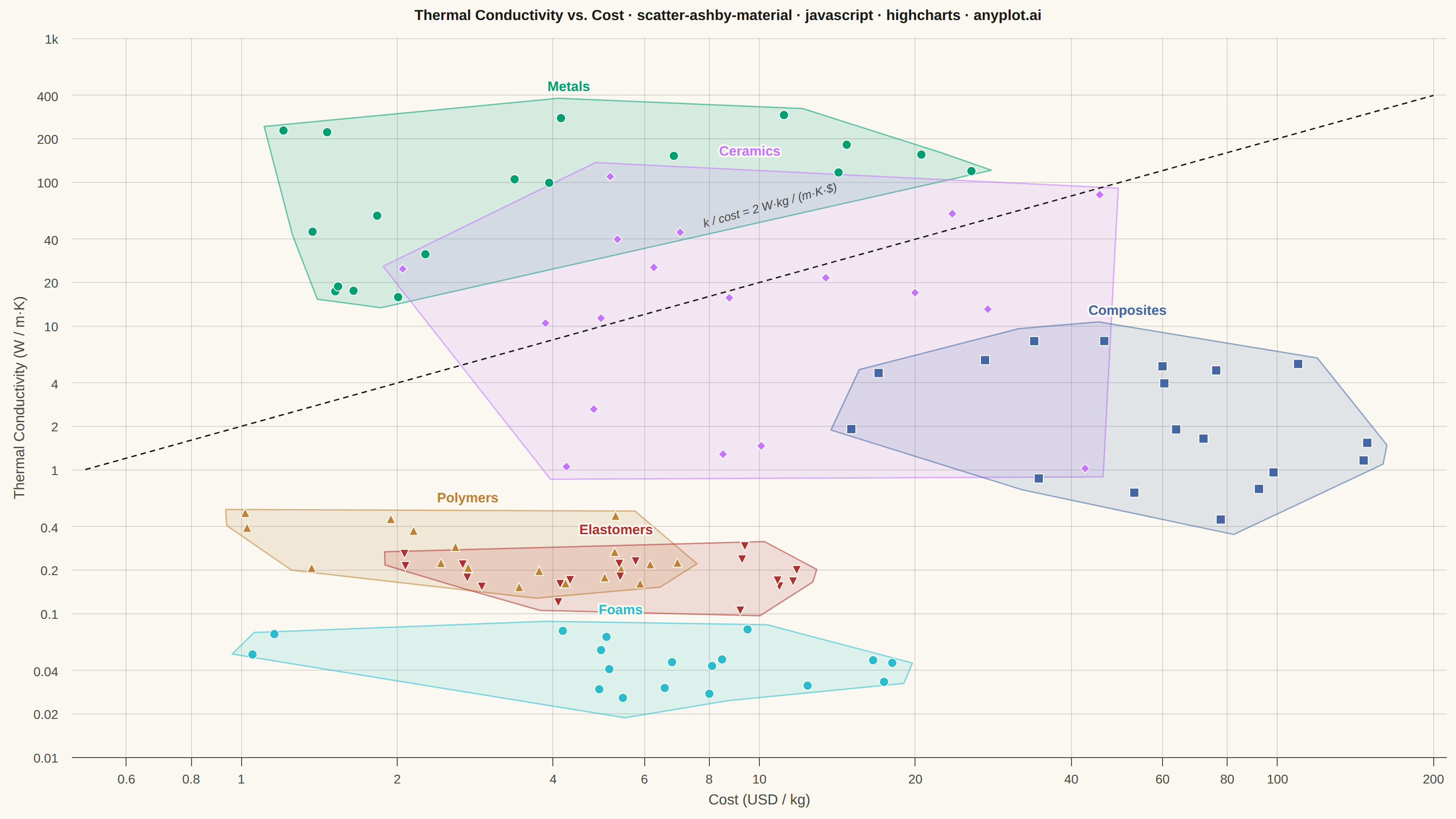
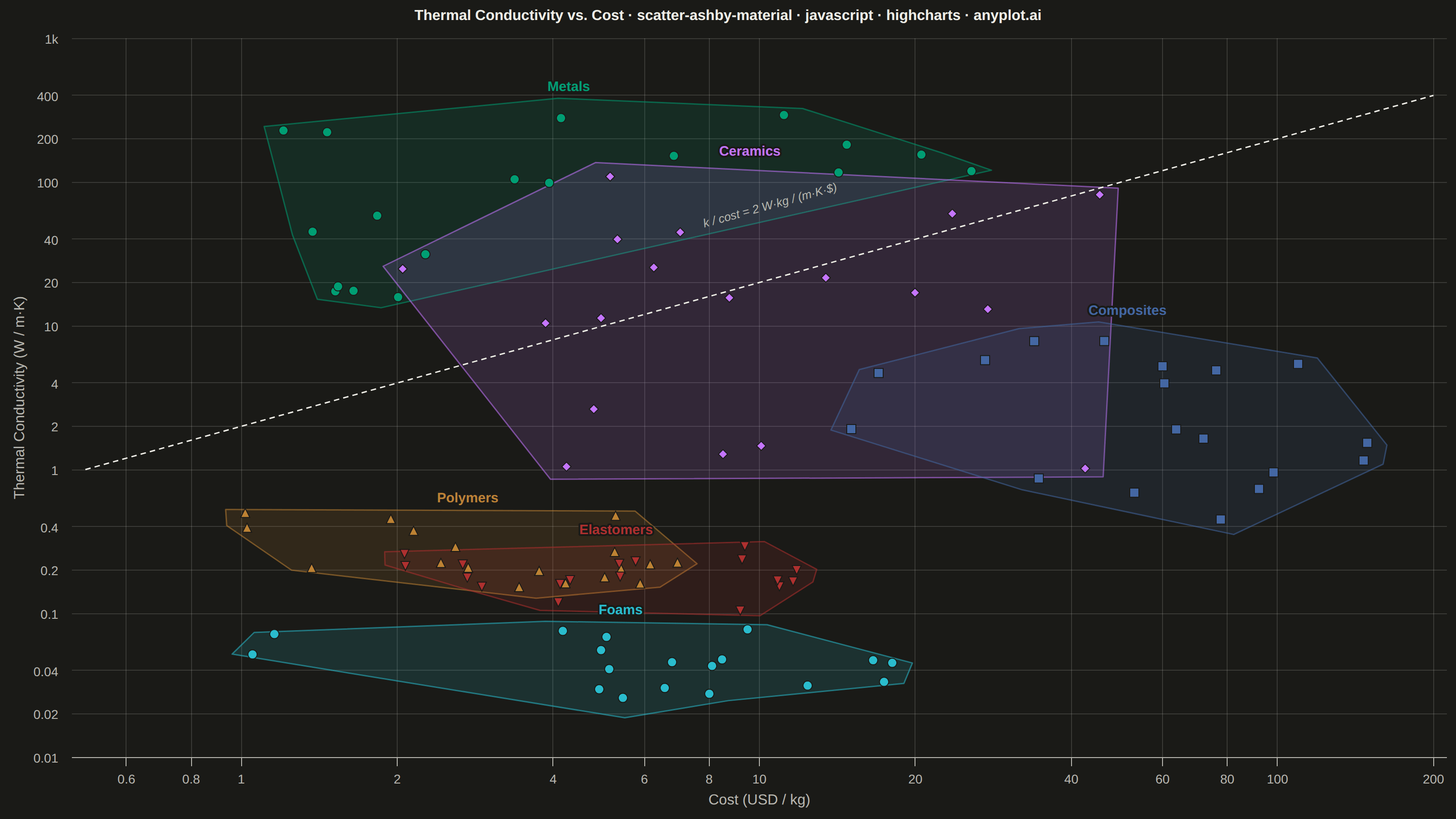
A log-log scatter plot comparing two material properties (e.g., Young's modulus vs. density) with material families displayed as labeled bubble regions. Developed by Michael Ashby for systematic material selection in engineering design, this chart enables rapid visual comparison of material classes across multiple property dimensions. It is a standard tool in materials science and mechanical engineering education.
// anyplot.ai
// scatter-ashby-material: Ashby Material Selection Chart
// Library: highcharts 12.6.0 | JavaScript 22.23.2
// Quality: 92/100 | Created: 2026-08-24

const t = window.ANYPLOT_TOKENS;

// --- Deterministic PRNG (LCG, 32-bit safe via Math.imul) -------------------
let seed = 42;
function rand() {
  seed = (Math.imul(1103515245, seed) + 12345) | 0;
  return (seed >>> 0) / 4294967296;
}
function logUniform(min, max) {
  const lo = Math.log10(min);
  const hi = Math.log10(max);
  return Math.pow(10, lo + rand() * (hi - lo));
}

// --- Data: cost vs. thermal conductivity, by material family ---------------
// (heat-exchanger material selection: want high conductivity at low cost)
const families = [
  { name: "Metals", xRange: [1, 30], yRange: [15, 400], count: 18,
    materials: ["Copper", "Aluminum Alloy", "Steel", "Titanium Alloy", "Brass", "Magnesium Alloy", "Nickel Alloy"] },
  { name: "Ceramics", xRange: [2, 50], yRange: [1, 150], count: 18,
    materials: ["Silicon Carbide", "Alumina", "Aluminum Nitride", "Zirconia", "Borosilicate Glass", "Silicon Nitride"] },
  { name: "Composites", xRange: [10, 150], yRange: [0.3, 8], count: 18,
    materials: ["CFRP", "GFRP", "Al-SiC MMC", "Kevlar Composite", "Plywood"] },
  { name: "Polymers", xRange: [1, 8], yRange: [0.15, 0.5], count: 18,
    materials: ["Polyethylene", "Polypropylene", "Nylon", "PVC", "Polycarbonate", "PTFE"] },
  { name: "Elastomers", xRange: [2, 15], yRange: [0.1, 0.3], count: 18,
    materials: ["Natural Rubber", "Silicone Rubber", "Neoprene", "EPDM", "Polyurethane Elastomer"] },
  { name: "Foams", xRange: [1, 20], yRange: [0.02, 0.09], count: 18,
    materials: ["Polyurethane Foam", "Polystyrene Foam", "Cork", "Metal Foam", "Mineral Wool"] },
];

families.forEach((f) => {
  f.points = Array.from({ length: f.count }, () => ({
    x: logUniform(f.xRange[0], f.xRange[1]),
    y: logUniform(f.yRange[0], f.yRange[1]),
    material: f.materials[Math.floor(rand() * f.materials.length)],
  }));
});

// --- Title (mandated format, fontsize scaled to length) --------------------
const title = "Thermal Conductivity vs. Cost · scatter-ashby-material · javascript · highcharts · anyplot.ai";
const titleFontSize = Math.max(15, Math.round(22 * Math.min(1, 67 / title.length)));

// --- Chart -------------------------------------------------------------------
const chart = Highcharts.chart("container", {
  chart: { type: "scatter", backgroundColor: "transparent", animation: false,
           style: { fontFamily: "inherit" } },
  credits: { enabled: false },
  colors: t.palette,
  title: { text: title, style: { color: t.ink, fontSize: `${titleFontSize}px`, fontWeight: "600" } },
  xAxis: { type: "logarithmic", gridLineWidth: 1, gridLineColor: t.grid,
           lineColor: t.inkSoft, tickColor: t.inkSoft,
           labels: { style: { color: t.inkSoft, fontSize: "14px" } },
           title: { text: "Cost (USD / kg)", style: { color: t.inkSoft, fontSize: "16px" } } },
  yAxis: { type: "logarithmic", gridLineWidth: 1, gridLineColor: t.grid,
           lineColor: t.inkSoft, tickColor: t.inkSoft,
           labels: { style: { color: t.inkSoft, fontSize: "14px" } },
           title: { text: "Thermal Conductivity (W / m·K)", style: { color: t.inkSoft, fontSize: "16px" } } },
  legend: { enabled: false },
  plotOptions: { series: { animation: false } },
  series: [
    ...families.map((f, i) => ({
      name: f.name,
      type: "scatter",
      color: t.palette[i],
      data: f.points.map((p) => ({ x: p.x, y: p.y, material: p.material })),
      marker: { radius: 5, lineColor: t.pageBg, lineWidth: 1 },
      tooltip: { pointFormat: "<b>{point.material}</b><br/>Cost: {point.x:.2f} $/kg<br/>k: {point.y:.3f} W/m·K" },
    })),
    {
      name: "Thermal value index",
      type: "line",
      color: t.ink,
      dashStyle: "Dash",
      lineWidth: 1.5,
      marker: { enabled: false },
      enableMouseTracking: false,
      data: [[0.5, 1], [200, 400]],
    },
  ],
});

// --- Family bubble regions: padded convex hulls + direct labels ------------
// Computed in pixel space (already log-transformed by the axes), so a straight
// monotone-chain hull reflects the visual point cloud, not the raw values.
function convexHull(pts) {
  const s = pts.slice().sort((a, b) => a[0] - b[0] || a[1] - b[1]);
  const cross = (o, a, b) => (a[0] - o[0]) * (b[1] - o[1]) - (a[1] - o[1]) * (b[0] - o[0]);
  const lower = [];
  for (const p of s) {
    while (lower.length >= 2 && cross(lower[lower.length - 2], lower[lower.length - 1], p) <= 0) lower.pop();
    lower.push(p);
  }
  const upper = [];
  for (let i = s.length - 1; i >= 0; i--) {
    const p = s[i];
    while (upper.length >= 2 && cross(upper[upper.length - 2], upper[upper.length - 1], p) <= 0) upper.pop();
    upper.push(p);
  }
  upper.pop();
  lower.pop();
  return lower.concat(upper);
}
function padHull(hull, pad) {
  const cx = hull.reduce((s, p) => s + p[0], 0) / hull.length;
  const cy = hull.reduce((s, p) => s + p[1], 0) / hull.length;
  return hull.map(([x, y]) => {
    const dx = x - cx;
    const dy = y - cy;
    const len = Math.sqrt(dx * dx + dy * dy) || 1;
    return [x + (dx / len) * pad, y + (dy / len) * pad];
  });
}

const xAxis = chart.xAxis[0];
const yAxis = chart.yAxis[0];
const hullGroup = chart.renderer.g("ashby-hulls").attr({ zIndex: 2 }).add();
const labelGroup = chart.renderer.g("ashby-labels").attr({ zIndex: 7 }).add();

families.forEach((f, i) => {
  const pixelPts = f.points.map((p) => [xAxis.toPixels(p.x, false), yAxis.toPixels(p.y, false)]);
  const hull = padHull(convexHull(pixelPts), 22);
  const path = hull.map(([x, y], idx) => `${idx === 0 ? "M" : "L"}${x},${y}`).join(" ") + " Z";
  const color = t.palette[i];
  chart.renderer
    .path()
    .attr({
      d: path,
      fill: Highcharts.color(color).setOpacity(0.14).get(),
      stroke: Highcharts.color(color).setOpacity(0.55).get(),
      "stroke-width": 1.5,
      "stroke-linejoin": "round",
    })
    .add(hullGroup);

  const topPoint = hull.reduce((top, p) => (p[1] < top[1] ? p : top), hull[0]);
  const cx = hull.reduce((s, p) => s + p[0], 0) / hull.length;
  chart.renderer
    .text(f.name, cx, topPoint[1] - 8)
    .attr({ align: "center", zIndex: 7 })
    .css({ color, fontSize: "15px", fontWeight: "600", textOutline: `2px ${t.pageBg}` })
    .add(labelGroup);
});

// --- Guide-line label, aligned to the line's on-screen slope ----------------
const gx1 = xAxis.toPixels(0.5, false);
const gy1 = yAxis.toPixels(1, false);
const gx2 = xAxis.toPixels(200, false);
const gy2 = yAxis.toPixels(400, false);
const guideAngle = (Math.atan2(gy2 - gy1, gx2 - gx1) * 180) / Math.PI;
chart.renderer
  .text("k / cost = 2 W·kg / (m·K·$)", (gx1 + gx2) / 2 - 60, (gy1 + gy2) / 2 - 60)
  .attr({ rotation: guideAngle, zIndex: 7 })
  .css({ color: t.inkSoft, fontSize: "13px", fontStyle: "italic" })
  .add(labelGroup);
Runnable source as JSON, for any HTTP client: https://api.anyplot.ai/specs/scatter-ashby-material/highcharts/code. Any spec id and library id listed in llms-full.txt fit the same URL shape; every URL below is complete and callable.
{
  "spec_id": "scatter-ashby-material",
  "language": "javascript",
  "library": "highcharts",
  "page": "https://anyplot.ai/scatter-ashby-material/javascript/highcharts",
  "hub": "https://anyplot.ai/scatter-ashby-material",
  "code_json": "https://api.anyplot.ai/specs/scatter-ashby-material/highcharts/code",
  "spec_json": "https://api.anyplot.ai/specs/scatter-ashby-material",
  "render_light_png": "https://storage.googleapis.com/anyplot-images/plots/scatter-ashby-material/javascript/highcharts/plot-light.png",
  "render_dark_png": "https://storage.googleapis.com/anyplot-images/plots/scatter-ashby-material/javascript/highcharts/plot-dark.png",
  "interactive_light_html": "https://storage.googleapis.com/anyplot-images/plots/scatter-ashby-material/javascript/highcharts/plot-light.html",
  "interactive_dark_html": "https://storage.googleapis.com/anyplot-images/plots/scatter-ashby-material/javascript/highcharts/plot-dark.html",
  "quality_score": 92.0,
  "license": "MIT",
  "guide": "https://anyplot.ai/llms.txt"
}
Part of Ashby Material Selection Chart on anyplot.ai.