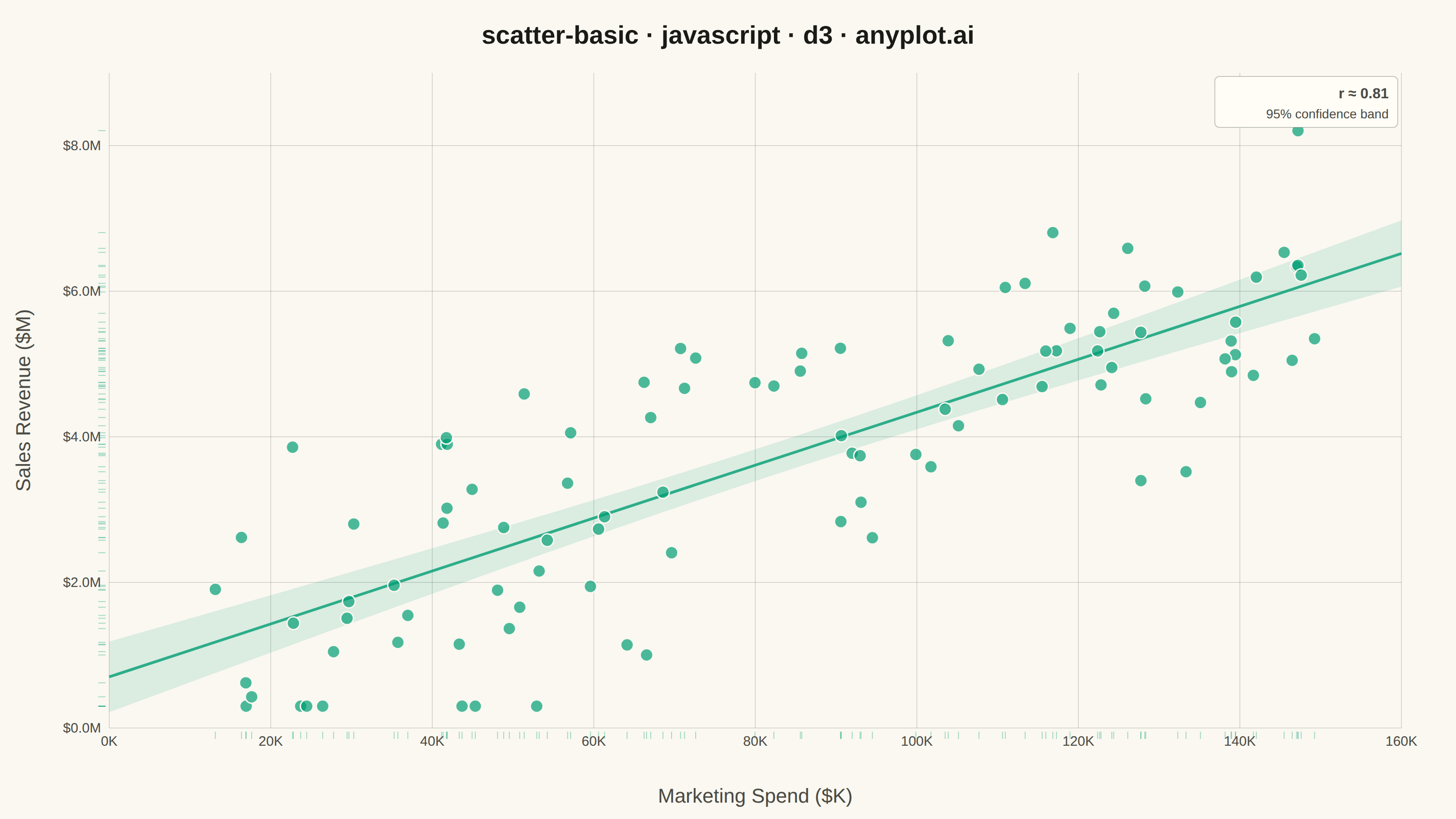
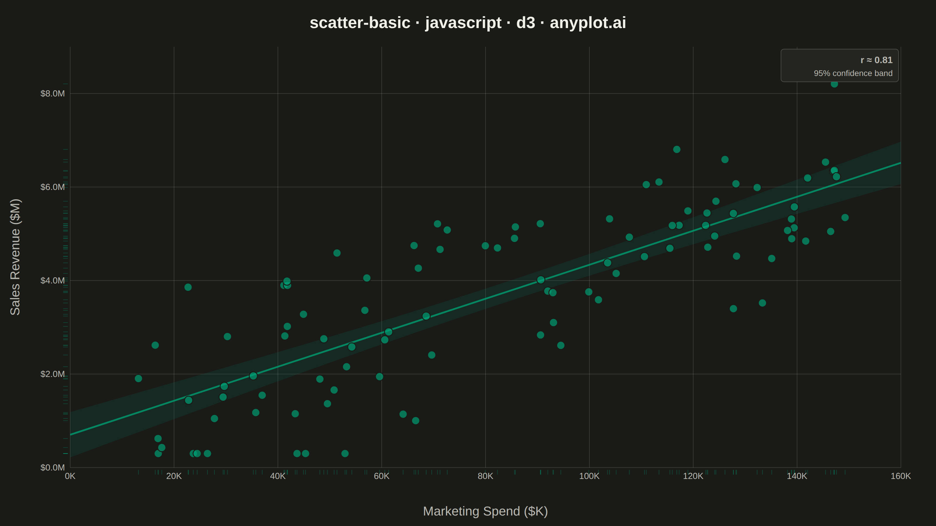
The same plot in 14 other libraries — JavaScript: Chart.js, Apache ECharts, Highcharts, MUI X Charts; Python: Altair, Bokeh, lets-plot, Matplotlib, Plotly, plotnine, Pygal, Seaborn; R: ggplot2; Julia: Makie.jl. Compare all 15 side by side: Basic Scatter Plot in Python, R, Julia and JavaScript.
A fundamental 2D scatter plot that displays the relationship between two numeric variables by plotting points on a Cartesian coordinate system. This visualization is essential for exploring correlations, identifying patterns, detecting outliers, and understanding the distribution of paired data points.
// anyplot.ai
// scatter-basic: Basic Scatter Plot
// Library: d3 7.9.0 | JavaScript 22.22.3
// Quality: 94/100 | Updated: 2026-06-25

const t = window.ANYPLOT_TOKENS;
const { width, height } = window.ANYPLOT_SIZE;
const margin = { top: 80, right: 60, bottom: 100, left: 120 };
const iw = width - margin.left - margin.right;
const ih = height - margin.top - margin.bottom;

// --- Data (deterministic LCG seed=42, marketing spend vs sales revenue) ----
let seed = 42;
function lcgRand() {
  seed = (1664525 * seed + 1013904223) >>> 0;
  return seed / 4294967296;
}
function lcgRandn() {
  const u1 = lcgRand() + 1e-10;
  const u2 = lcgRand();
  return Math.sqrt(-2 * Math.log(u1)) * Math.cos(2 * Math.PI * u2);
}

const data = Array.from({ length: 100 }, () => {
  const spend = 10 + lcgRand() * 140;
  const sales = Math.max(0.3, 0.8 + spend * 0.035 + lcgRandn() * 1.2);
  return { x: spend, y: sales };
});

// --- OLS regression and Pearson r ------------------------------------------
const n = data.length;
const sumX = data.reduce((s, d) => s + d.x, 0);
const sumY = data.reduce((s, d) => s + d.y, 0);
const sumXY = data.reduce((s, d) => s + d.x * d.y, 0);
const sumX2 = data.reduce((s, d) => s + d.x * d.x, 0);
const sumY2 = data.reduce((s, d) => s + d.y * d.y, 0);
const slope = (n * sumXY - sumX * sumY) / (n * sumX2 - sumX * sumX);
const intercept = (sumY - slope * sumX) / n;
const r = (n * sumXY - sumX * sumY) /
  Math.sqrt((n * sumX2 - sumX * sumX) * (n * sumY2 - sumY * sumY));

// --- 95% CI band statistics ------------------------------------------------
const xMean = sumX / n;
const sxx = data.reduce((s, d) => s + (d.x - xMean) ** 2, 0);
const sse = data.reduce((s, d) => {
  const yhat = intercept + slope * d.x;
  return s + (d.y - yhat) ** 2;
}, 0);
const see = Math.sqrt(sse / (n - 2));
const tCrit = 1.984; // t(98, 0.975) for 95% CI

// --- SVG mount -------------------------------------------------------------
const svg = d3.select("#container")
  .append("svg")
  .attr("width", width)
  .attr("height", height);
const g = svg.append("g").attr("transform", `translate(${margin.left},${margin.top})`);

// --- Scales ----------------------------------------------------------------
const x = d3.scaleLinear()
  .domain([0, d3.max(data, (d) => d.x) * 1.04]).nice().range([0, iw]);
const y = d3.scaleLinear()
  .domain([0, d3.max(data, (d) => d.y) * 1.04]).nice().range([ih, 0]);

// --- Grid lines (both axes, floating-grid — no domain line) ----------------
g.append("g").attr("transform", `translate(0,${ih})`)
  .call(d3.axisBottom(x).ticks(8).tickSize(-ih).tickFormat(""))
  .call((ax) => ax.select(".domain").remove())
  .call((ax) => ax.selectAll("line").attr("stroke", t.grid));

g.append("g")
  .call(d3.axisLeft(y).ticks(6).tickSize(-iw).tickFormat(""))
  .call((ax) => ax.select(".domain").remove())
  .call((ax) => ax.selectAll("line").attr("stroke", t.grid));

// --- 95% CI band using d3.area() (D3-native analytical layer) --------------
const xDom = x.domain();
const bandData = d3.range(0, 101).map((i) => {
  const xv = xDom[0] + (xDom[1] - xDom[0]) * i / 100;
  const yhat = intercept + slope * xv;
  const ci = tCrit * see * Math.sqrt(1 / n + (xv - xMean) ** 2 / sxx);
  return { x: xv, y0: Math.max(0, yhat - ci), y1: yhat + ci };
});

g.append("path")
  .datum(bandData)
  .attr("fill", t.palette[0])
  .attr("fill-opacity", 0.12)
  .attr("stroke", "none")
  .attr("d", d3.area()
    .x((d) => x(d.x))
    .y0((d) => y(d.y0))
    .y1((d) => y(d.y1)));

// --- OLS trend line --------------------------------------------------------
g.append("path")
  .datum([
    { x: xDom[0], y: intercept + slope * xDom[0] },
    { x: xDom[1], y: intercept + slope * xDom[1] },
  ])
  .attr("fill", "none")
  .attr("stroke", t.palette[0])
  .attr("stroke-width", 3)
  .attr("stroke-opacity", 0.8)
  .attr("d", d3.line().x((d) => x(d.x)).y((d) => y(d.y)));

// --- Marginal rug marks (subtle distribution indicators on both axes) ------
g.selectAll(".rug-x").data(data).join("line")
  .attr("class", "rug-x")
  .attr("x1", (d) => x(d.x)).attr("x2", (d) => x(d.x))
  .attr("y1", ih + 4).attr("y2", ih + 12)
  .attr("stroke", t.palette[0]).attr("stroke-opacity", 0.35).attr("stroke-width", 1);

g.selectAll(".rug-y").data(data).join("line")
  .attr("class", "rug-y")
  .attr("x1", -4).attr("x2", -12)
  .attr("y1", (d) => y(d.y)).attr("y2", (d) => y(d.y))
  .attr("stroke", t.palette[0]).attr("stroke-opacity", 0.35).attr("stroke-width", 1);

// --- Scatter markers -------------------------------------------------------
g.selectAll("circle").data(data).join("circle")
  .attr("cx", (d) => x(d.x))
  .attr("cy", (d) => y(d.y))
  .attr("r", 7)
  .attr("fill", t.palette[0])
  .attr("fill-opacity", 0.7)
  .attr("stroke", t.pageBg)
  .attr("stroke-width", 1.5);

// --- X axis (floating — domain removed for clean open look) ----------------
g.append("g").attr("transform", `translate(0,${ih})`)
  .call(d3.axisBottom(x).ticks(8).tickFormat((d) => `${d}K`))
  .call((ax) => ax.select(".domain").remove())
  .call((ax) => ax.selectAll(".tick text").attr("fill", t.inkSoft).style("font-size", "15px"))
  .call((ax) => ax.selectAll(".tick line").remove());

// --- Y axis (floating — domain removed for clean open look) ----------------
g.append("g")
  .call(d3.axisLeft(y).ticks(6).tickFormat((d) => `$${d.toFixed(1)}M`))
  .call((ax) => ax.select(".domain").remove())
  .call((ax) => ax.selectAll(".tick text").attr("fill", t.inkSoft).style("font-size", "15px"))
  .call((ax) => ax.selectAll(".tick line").remove());

// --- Correlation + CI annotation with elevated-bg callout box (upper-right)
const annotG = g.append("g");
annotG.append("rect")
  .attr("x", iw - 205).attr("y", 4)
  .attr("width", 201).attr("height", 56)
  .attr("rx", 5).attr("ry", 5)
  .attr("fill", t.elevatedBg)
  .attr("stroke", t.inkSoft)
  .attr("stroke-opacity", 0.3)
  .attr("stroke-width", 1);
annotG.append("text")
  .attr("x", iw - 14).attr("y", 28)
  .attr("text-anchor", "end")
  .attr("fill", t.inkSoft)
  .style("font-size", "16px").style("font-weight", "600")
  .text(`r ≈ ${r.toFixed(2)}`);
annotG.append("text")
  .attr("x", iw - 14).attr("y", 50)
  .attr("text-anchor", "end")
  .attr("fill", t.inkSoft)
  .style("font-size", "14px")
  .text("95% confidence band");

// --- Axis labels -----------------------------------------------------------
svg.append("text")
  .attr("x", margin.left + iw / 2).attr("y", height - 18)
  .attr("text-anchor", "middle").attr("fill", t.inkSoft)
  .style("font-size", "22px").text("Marketing Spend ($K)");

svg.append("text")
  .attr("transform", `translate(33,${margin.top + ih / 2}) rotate(-90)`)
  .attr("text-anchor", "middle").attr("fill", t.inkSoft)
  .style("font-size", "22px").text("Sales Revenue ($M)");

// --- Title -----------------------------------------------------------------
svg.append("text")
  .attr("x", width / 2).attr("y", 48)
  .attr("text-anchor", "middle").attr("fill", t.ink)
  .style("font-size", "28px").style("font-weight", "600")
  .text("scatter-basic · javascript · d3 · anyplot.ai");
Runnable source as JSON, for any HTTP client: https://api.anyplot.ai/specs/scatter-basic/d3/code. Any spec id and library id listed in llms-full.txt fit the same URL shape; every URL below is complete and callable.
{
  "spec_id": "scatter-basic",
  "language": "javascript",
  "library": "d3",
  "page": "https://anyplot.ai/scatter-basic/javascript/d3",
  "hub": "https://anyplot.ai/scatter-basic",
  "code_json": "https://api.anyplot.ai/specs/scatter-basic/d3/code",
  "spec_json": "https://api.anyplot.ai/specs/scatter-basic",
  "render_light_png": "https://storage.googleapis.com/anyplot-images/plots/scatter-basic/javascript/d3/plot-light.png",
  "render_dark_png": "https://storage.googleapis.com/anyplot-images/plots/scatter-basic/javascript/d3/plot-dark.png",
  "interactive_light_html": "https://storage.googleapis.com/anyplot-images/plots/scatter-basic/javascript/d3/plot-light.html",
  "interactive_dark_html": "https://storage.googleapis.com/anyplot-images/plots/scatter-basic/javascript/d3/plot-dark.html",
  "quality_score": 94.0,
  "license": "MIT",
  "guide": "https://anyplot.ai/llms.txt"
}
Part of Basic Scatter Plot on anyplot.ai.