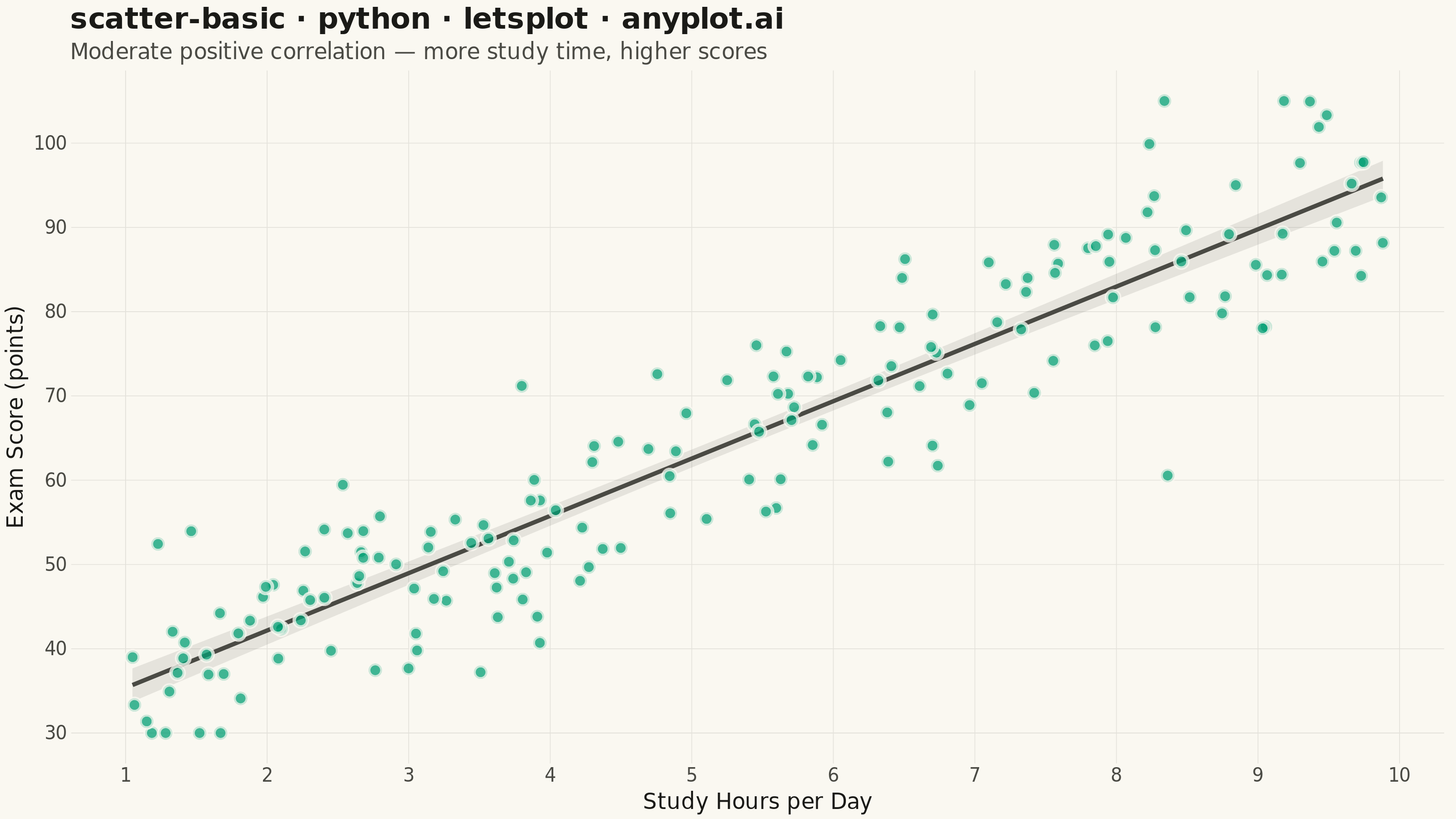
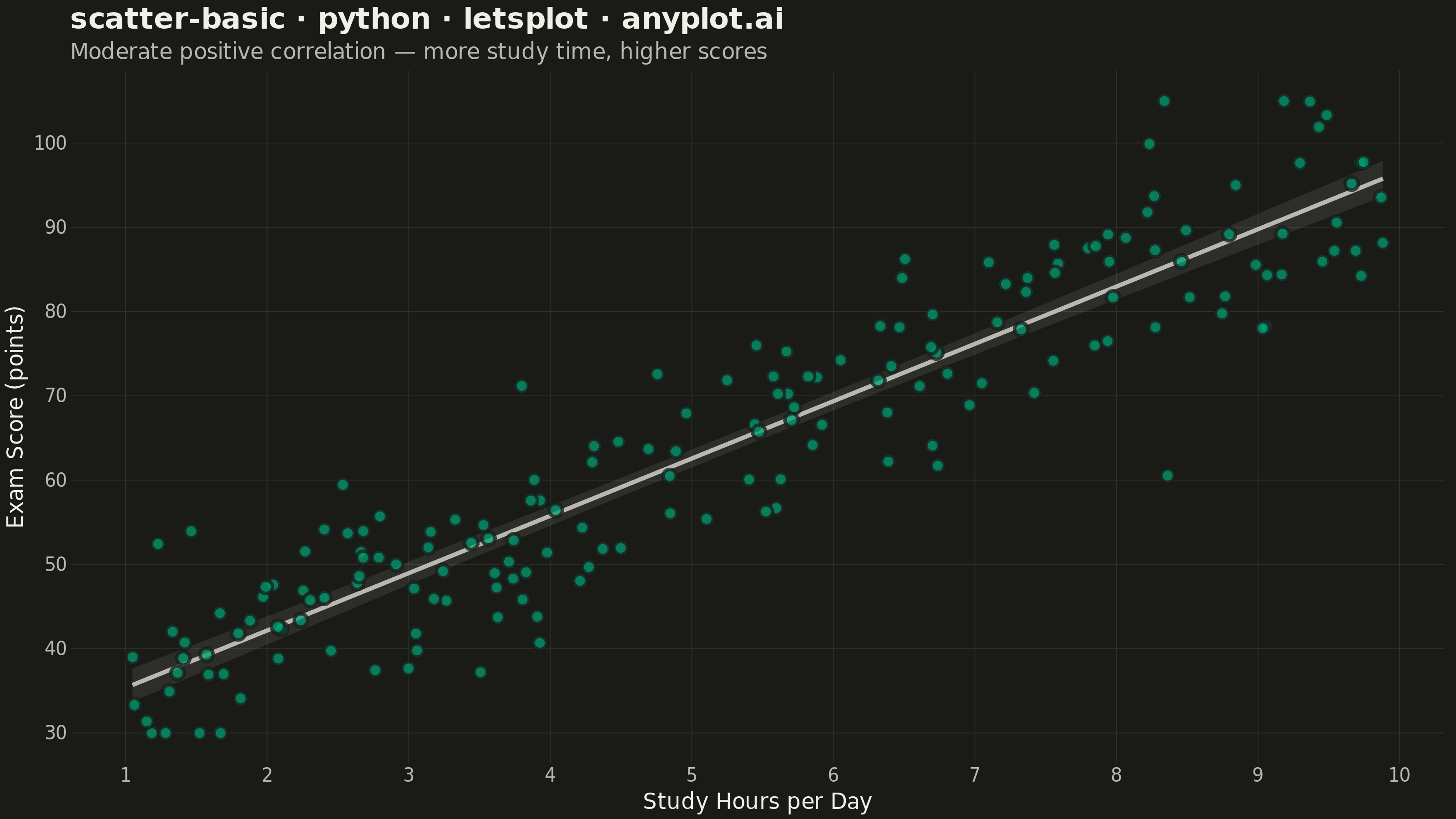
A fundamental 2D scatter plot that displays the relationship between two numeric variables by plotting points on a Cartesian coordinate system. This visualization is essential for exploring correlations, identifying patterns, detecting outliers, and understanding the distribution of paired data points.
""" anyplot.ai
scatter-basic: Basic Scatter Plot
Library: letsplot 4.10.1 | Python 3.13.14
Quality: 92/100 | Updated: 2026-06-25
"""

import os

import numpy as np
import pandas as pd
from lets_plot import (
    LetsPlot,
    aes,
    element_blank,
    element_line,
    element_rect,
    element_text,
    geom_point,
    geom_smooth,
    ggplot,
    ggsize,
    labs,
    layer_tooltips,
    theme,
    theme_minimal,
)
from lets_plot.export import ggsave


LetsPlot.setup_html()

# Theme tokens
THEME = os.getenv("ANYPLOT_THEME", "light")
PAGE_BG = "#FAF8F1" if THEME == "light" else "#1A1A17"
INK = "#1A1A17" if THEME == "light" else "#F0EFE8"
INK_SOFT = "#4A4A44" if THEME == "light" else "#B8B7B0"
# Pre-blended ~10% INK over PAGE_BG (element_line has no alpha in lets-plot)
GRID = "#E4E2DB" if THEME == "light" else "#2F2F2C"
BRAND = "#009E73"  # Imprint palette position 1

# Data — study hours vs exam scores (moderate positive correlation ~0.7)
np.random.seed(42)
study_hours = np.random.uniform(1.0, 10.0, 180)
exam_scores = study_hours * 6.8 + np.random.normal(0, 7.5, 180) + 28
exam_scores = np.clip(exam_scores, 30, 105)
df = pd.DataFrame({"study_hours": study_hours, "exam_scores": exam_scores})

# Plot — linear trend beneath points guides the eye to the correlation
plot = (
    ggplot(df, aes(x="study_hours", y="exam_scores"))
    + geom_smooth(method="lm", se=True, color=INK_SOFT, fill=INK_SOFT, alpha=0.12, size=1.0)
    + geom_point(
        shape=21,
        fill=BRAND,
        color=PAGE_BG,
        size=2.5,
        alpha=0.75,
        stroke=0.8,
        tooltips=layer_tooltips().line("Study Hours: @study_hours h").line("Exam Score: @exam_scores pts"),
    )
    + labs(
        x="Study Hours per Day",
        y="Exam Score (points)",
        title="scatter-basic · python · letsplot · anyplot.ai",
        subtitle="Moderate positive correlation — more study time, higher scores",
    )
    + ggsize(800, 450)
    + theme_minimal()
    + theme(
        plot_background=element_rect(fill=PAGE_BG, color=PAGE_BG),
        panel_background=element_rect(fill=PAGE_BG, color=PAGE_BG),
        panel_grid_major=element_line(color=GRID, size=0.4),
        panel_grid_minor=element_blank(),
        axis_title=element_text(size=12, color=INK),
        axis_text=element_text(size=10, color=INK_SOFT),
        axis_line=element_line(color=INK_SOFT, size=0.4),
        axis_ticks=element_blank(),
        plot_title=element_text(size=16, color=INK, face="bold"),
        plot_subtitle=element_text(size=12, color=INK_SOFT),
    )
)

# Save — ggsize(800, 450) × scale=4 → 3200 × 1800 px
ggsave(plot, filename=f"plot-{THEME}.png", path=".", scale=4)
ggsave(plot, filename=f"plot-{THEME}.html", path=".")
Runnable source as JSON, for any HTTP client: https://api.anyplot.ai/specs/scatter-basic/letsplot/code. Any spec id and library id listed in llms-full.txt fit the same URL shape; every URL below is complete and callable.
{
  "spec_id": "scatter-basic",
  "language": "python",
  "library": "letsplot",
  "page": "https://anyplot.ai/scatter-basic/python/letsplot",
  "hub": "https://anyplot.ai/scatter-basic",
  "code_json": "https://api.anyplot.ai/specs/scatter-basic/letsplot/code",
  "spec_json": "https://api.anyplot.ai/specs/scatter-basic",
  "render_light_png": "https://storage.googleapis.com/anyplot-images/plots/scatter-basic/python/letsplot/plot-light.png",
  "render_dark_png": "https://storage.googleapis.com/anyplot-images/plots/scatter-basic/python/letsplot/plot-dark.png",
  "interactive_light_html": "https://storage.googleapis.com/anyplot-images/plots/scatter-basic/python/letsplot/plot-light.html",
  "interactive_dark_html": "https://storage.googleapis.com/anyplot-images/plots/scatter-basic/python/letsplot/plot-dark.html",
  "quality_score": 92.0,
  "license": "MIT",
  "guide": "https://anyplot.ai/llms.txt"
}
Part of Basic Scatter Plot on anyplot.ai.