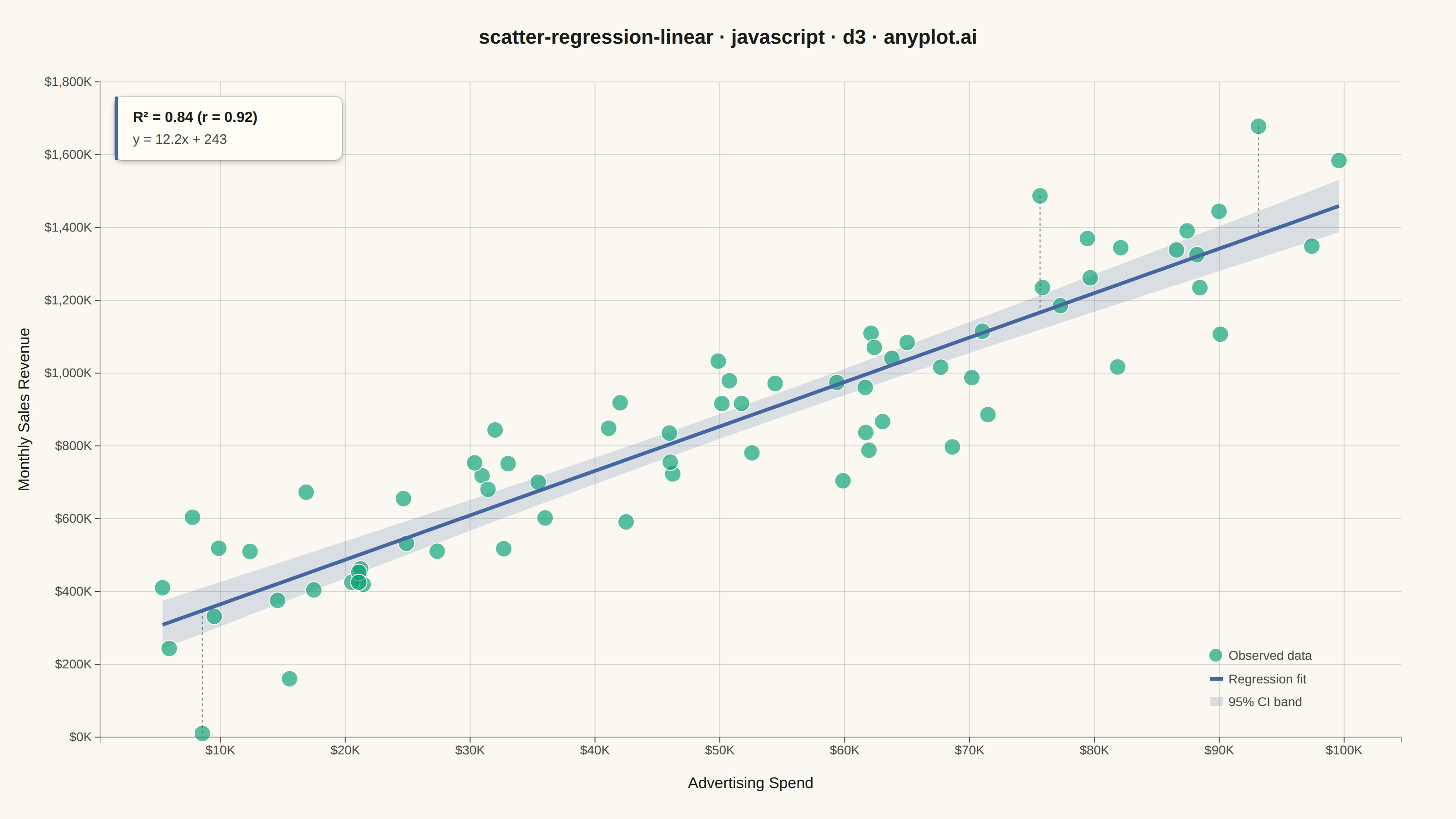
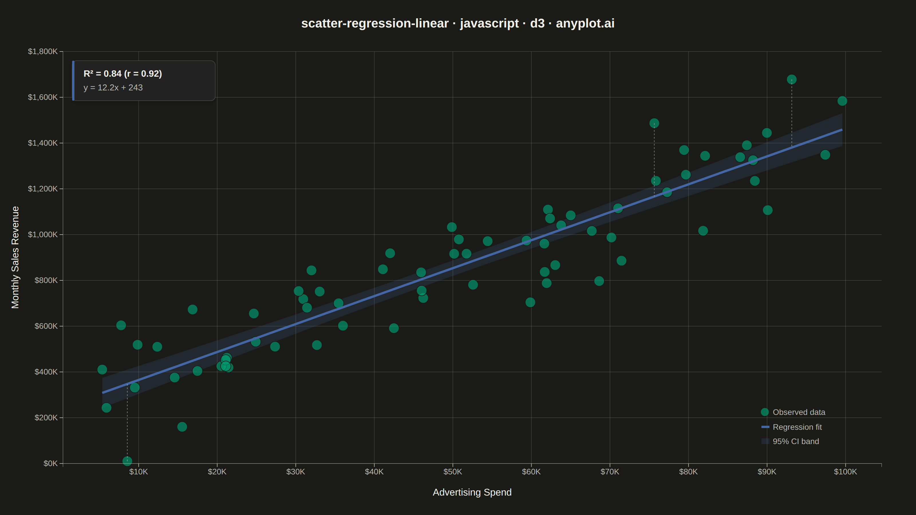
The same plot in 14 other libraries — JavaScript: Chart.js, Apache ECharts, Highcharts, MUI X Charts; Python: Altair, Bokeh, lets-plot, Matplotlib, Plotly, plotnine, Pygal, Seaborn; R: ggplot2; Julia: Makie.jl. Compare all 15 side by side: Scatter Plot with Linear Regression in Python, R, Julia and JavaScript.
A scatter plot that displays the relationship between two numeric variables with a fitted linear regression line and confidence interval band. This visualization extends the basic scatter plot by adding statistical modeling elements, making it ideal for understanding linear relationships, assessing model fit, and communicating the strength of correlations with visual uncertainty quantification.
// anyplot.ai
// scatter-regression-linear: Scatter Plot with Linear Regression
// Library: d3 7.9.0 | JavaScript 22.23.1
// Quality: 90/100 | Created: 2026-08-05

const t = window.ANYPLOT_TOKENS;
const { width, height } = window.ANYPLOT_SIZE;
const margin = { top: 90, right: 60, bottom: 90, left: 110 };
const iw = width - margin.left - margin.right;
const ih = height - margin.top - margin.bottom;

// --- Data (in-memory, deterministic, seeded LCG) ----------------------------
// mulberry32: small fixed-seed PRNG (the browser has no seeded Math.random)
const rand = (() => {
  let a = 42;
  return () => {
    a |= 0;
    a = (a + 0x6d2b79f5) | 0;
    let r = Math.imul(a ^ (a >>> 15), 1 | a);
    r = (r + Math.imul(r ^ (r >>> 7), 61 | r)) ^ r;
    return ((r ^ (r >>> 14)) >>> 0) / 4294967296;
  };
})();

const n = 70;
const trueSlope = 12;
const trueIntercept = 250;
const noiseStd = 150;
const data = [];
for (let i = 0; i < n; i++) {
  const adSpend = 5 + rand() * 95; // $ thousands
  const u1 = rand();
  const u2 = rand();
  const gaussian = Math.sqrt(-2 * Math.log(u1)) * Math.cos(2 * Math.PI * u2);
  const salesRevenue = trueSlope * adSpend + trueIntercept + gaussian * noiseStd;
  data.push({ x: adSpend, y: salesRevenue });
}

// --- Linear regression (ordinary least squares) -----------------------------
const xBar = d3.mean(data, (d) => d.x);
const yBar = d3.mean(data, (d) => d.y);
const sXX = d3.sum(data, (d) => (d.x - xBar) ** 2);
const sYY = d3.sum(data, (d) => (d.y - yBar) ** 2);
const sXY = d3.sum(data, (d) => (d.x - xBar) * (d.y - yBar));
const slope = sXY / sXX;
const intercept = yBar - slope * xBar;
const r = sXY / Math.sqrt(sXX * sYY);
const rSquared = r * r;
const dof = n - 2;
const sse = d3.sum(data, (d) => (d.y - (slope * d.x + intercept)) ** 2);
const stdError = Math.sqrt(sse / dof);
const tValue = 2.0; // two-tailed 95% CI, df ~68 (t-table converges near 2.0)

const xExtent = d3.extent(data, (d) => d.x);
const fitLine = d3.range(0, 101).map((i) => {
  const x = xExtent[0] + ((xExtent[1] - xExtent[0]) * i) / 100;
  const yHat = slope * x + intercept;
  const margin95 = tValue * stdError * Math.sqrt(1 / n + (x - xBar) ** 2 / sXX);
  return { x, yHat, yLow: yHat - margin95, yHigh: yHat + margin95 };
});

// --- Scales -------------------------------------------------------------------
const x = d3
  .scaleLinear()
  .domain([xExtent[0] - 5, xExtent[1] + 5])
  .range([0, iw]);
const yDomainMin = Math.min(d3.min(fitLine, (d) => d.yLow), d3.min(data, (d) => d.y));
const yDomainMax = Math.max(d3.max(fitLine, (d) => d.yHigh), d3.max(data, (d) => d.y));
const y = d3
  .scaleLinear()
  .domain([yDomainMin, yDomainMax])
  .nice()
  .range([ih, 0]);

// --- SVG mount ----------------------------------------------------------------
const svg = d3.select("#container").append("svg").attr("width", width).attr("height", height);
const g = svg.append("g").attr("transform", `translate(${margin.left},${margin.top})`);

// A soft drop-shadow filter (d3-authored SVG defs) gives the stats callout a
// subtle elevated feel instead of a flat rect-on-rect look.
const defs = svg.append("defs");
defs
  .append("filter")
  .attr("id", "stats-shadow")
  .attr("x", "-20%")
  .attr("y", "-20%")
  .attr("width", "140%")
  .attr("height", "140%")
  .append("feDropShadow")
  .attr("dx", 0)
  .attr("dy", 2)
  .attr("stdDeviation", 3)
  .attr("flood-color", "#000000")
  .attr("flood-opacity", 0.28);

// --- Gridlines ------------------------------------------------------------
g.append("g")
  .attr("transform", `translate(0,${ih})`)
  .call(d3.axisBottom(x).ticks(8).tickSize(-ih).tickFormat(""))
  .call((sel) => sel.select(".domain").remove())
  .selectAll("line")
  .attr("stroke", t.grid);
g.append("g")
  .call(d3.axisLeft(y).ticks(6).tickSize(-iw).tickFormat(""))
  .call((sel) => sel.select(".domain").remove())
  .selectAll("line")
  .attr("stroke", t.grid);

// --- Confidence band (95%) -----------------------------------------------
const area = d3
  .area()
  .x((d) => x(d.x))
  .y0((d) => y(d.yLow))
  .y1((d) => y(d.yHigh))
  .curve(d3.curveLinear);
g.append("path").datum(fitLine).attr("d", area).attr("fill", t.palette[2]).attr("opacity", 0.18);

// --- Scatter points ---------------------------------------------------------
g.selectAll("circle")
  .data(data)
  .join("circle")
  .attr("cx", (d) => x(d.x))
  .attr("cy", (d) => y(d.y))
  .attr("r", 9)
  .attr("fill", t.palette[0])
  .attr("fill-opacity", 0.65)
  .attr("stroke", t.pageBg)
  .attr("stroke-width", 1);

// --- Regression line --------------------------------------------------------
const line = d3
  .line()
  .x((d) => x(d.x))
  .y((d) => y(d.yHat));
g.append("path")
  .datum(fitLine)
  .attr("d", line)
  .attr("fill", "none")
  .attr("stroke", t.palette[2])
  .attr("stroke-width", 4);

// --- Residual callouts (d3-specific: sort + join to surface the largest
// deviations from the fit, giving the trend a concrete storytelling anchor) --
const topResiduals = data
  .map((d) => ({ ...d, yHat: slope * d.x + intercept }))
  .sort((a, b) => Math.abs(b.y - b.yHat) - Math.abs(a.y - a.yHat))
  .slice(0, 3);
g.selectAll(".residual-line")
  .data(topResiduals)
  .join("line")
  .attr("class", "residual-line")
  .attr("x1", (d) => x(d.x))
  .attr("y1", (d) => y(d.y))
  .attr("x2", (d) => x(d.x))
  .attr("y2", (d) => y(d.yHat))
  .attr("stroke", t.inkSoft)
  .attr("stroke-width", 1.25)
  .attr("stroke-dasharray", "3,3")
  .attr("stroke-opacity", 0.55);

// --- Axes ---------------------------------------------------------------------
const xAxis = g
  .append("g")
  .attr("transform", `translate(0,${ih})`)
  .call(d3.axisBottom(x).ticks(8).tickFormat((d) => `$${d}K`));
const yAxis = g.append("g").call(d3.axisLeft(y).ticks(6).tickFormat((d) => `$${d3.format(",")(Math.round(d))}K`));
for (const ax of [xAxis, yAxis]) {
  ax.selectAll("text").attr("fill", t.inkSoft).style("font-size", "14px");
  ax.selectAll("line").attr("stroke", t.inkSoft);
  ax.select(".domain").attr("stroke", t.inkSoft).attr("stroke-opacity", 0.5);
}

// --- Axis labels ---------------------------------------------------------------
g.append("text")
  .attr("x", iw / 2)
  .attr("y", ih + 56)
  .attr("text-anchor", "middle")
  .attr("fill", t.ink)
  .style("font-size", "17px")
  .text("Advertising Spend");
g.append("text")
  .attr("transform", "rotate(-90)")
  .attr("x", -ih / 2)
  .attr("y", -78)
  .attr("text-anchor", "middle")
  .attr("fill", t.ink)
  .style("font-size", "17px")
  .text("Monthly Sales Revenue");

// --- Fit statistics annotation (spec asks R²/r to be shown prominently) -------
const statsBox = g.append("g").attr("transform", "translate(16, 16)");
statsBox
  .append("rect")
  .attr("width", 250)
  .attr("height", 70)
  .attr("fill", t.elevatedBg)
  .attr("stroke", t.grid)
  .attr("stroke-width", 1)
  .attr("rx", 8)
  .style("filter", "url(#stats-shadow)");
statsBox.append("rect").attr("width", 4).attr("height", 70).attr("fill", t.palette[2]).attr("rx", 2);
statsBox
  .append("text")
  .attr("x", 20)
  .attr("y", 28)
  .attr("fill", t.ink)
  .style("font-size", "16px")
  .style("font-weight", "600")
  .text(`R² = ${rSquared.toFixed(2)}  (r = ${r.toFixed(2)})`);
statsBox
  .append("text")
  .attr("x", 20)
  .attr("y", 52)
  .attr("fill", t.inkSoft)
  .style("font-size", "15px")
  .text(`y = ${slope.toFixed(1)}x + ${intercept.toFixed(0)}`);

// --- Legend -------------------------------------------------------------------
const legend = g.append("g").attr("transform", `translate(${iw - 210}, ${ih - 90})`);
legend
  .append("circle")
  .attr("cx", 6)
  .attr("cy", 0)
  .attr("r", 7)
  .attr("fill", t.palette[0])
  .attr("fill-opacity", 0.65);
legend.append("text").attr("x", 20).attr("y", 5).attr("fill", t.inkSoft).style("font-size", "14px").text("Observed data");
legend
  .append("line")
  .attr("x1", 0)
  .attr("x2", 14)
  .attr("y1", 26)
  .attr("y2", 26)
  .attr("stroke", t.palette[2])
  .attr("stroke-width", 4);
legend.append("text").attr("x", 20).attr("y", 31).attr("fill", t.inkSoft).style("font-size", "14px").text("Regression fit");
legend.append("rect").attr("x", 0).attr("y", 46).attr("width", 14).attr("height", 10).attr("fill", t.palette[2]).attr("opacity", 0.18);
legend.append("text").attr("x", 20).attr("y", 56).attr("fill", t.inkSoft).style("font-size", "14px").text("95% CI band");

// --- Title ----------------------------------------------------------------------
svg
  .append("text")
  .attr("x", width / 2)
  .attr("y", 48)
  .attr("text-anchor", "middle")
  .attr("fill", t.ink)
  .style("font-size", "22px")
  .style("font-weight", "600")
  .text("scatter-regression-linear · javascript · d3 · anyplot.ai");
Runnable source as JSON, for any HTTP client: https://api.anyplot.ai/specs/scatter-regression-linear/d3/code. Any spec id and library id listed in llms-full.txt fit the same URL shape; every URL below is complete and callable.
{
  "spec_id": "scatter-regression-linear",
  "language": "javascript",
  "library": "d3",
  "page": "https://anyplot.ai/scatter-regression-linear/javascript/d3",
  "hub": "https://anyplot.ai/scatter-regression-linear",
  "code_json": "https://api.anyplot.ai/specs/scatter-regression-linear/d3/code",
  "spec_json": "https://api.anyplot.ai/specs/scatter-regression-linear",
  "render_light_png": "https://storage.googleapis.com/anyplot-images/plots/scatter-regression-linear/javascript/d3/plot-light.png",
  "render_dark_png": "https://storage.googleapis.com/anyplot-images/plots/scatter-regression-linear/javascript/d3/plot-dark.png",
  "interactive_light_html": "https://storage.googleapis.com/anyplot-images/plots/scatter-regression-linear/javascript/d3/plot-light.html",
  "interactive_dark_html": "https://storage.googleapis.com/anyplot-images/plots/scatter-regression-linear/javascript/d3/plot-dark.html",
  "quality_score": 90.0,
  "license": "MIT",
  "guide": "https://anyplot.ai/llms.txt"
}
Part of Scatter Plot with Linear Regression on anyplot.ai.