The same plot in 14 other libraries — Python: Altair, Bokeh, lets-plot, Matplotlib, Plotly, plotnine, Pygal, Seaborn; Julia: Makie.jl; JavaScript: Chart.js, D3.js, Apache ECharts, Highcharts, MUI X Charts. Compare all 15 side by side: Scatter Plot with Linear Regression in Python, R, Julia and JavaScript.
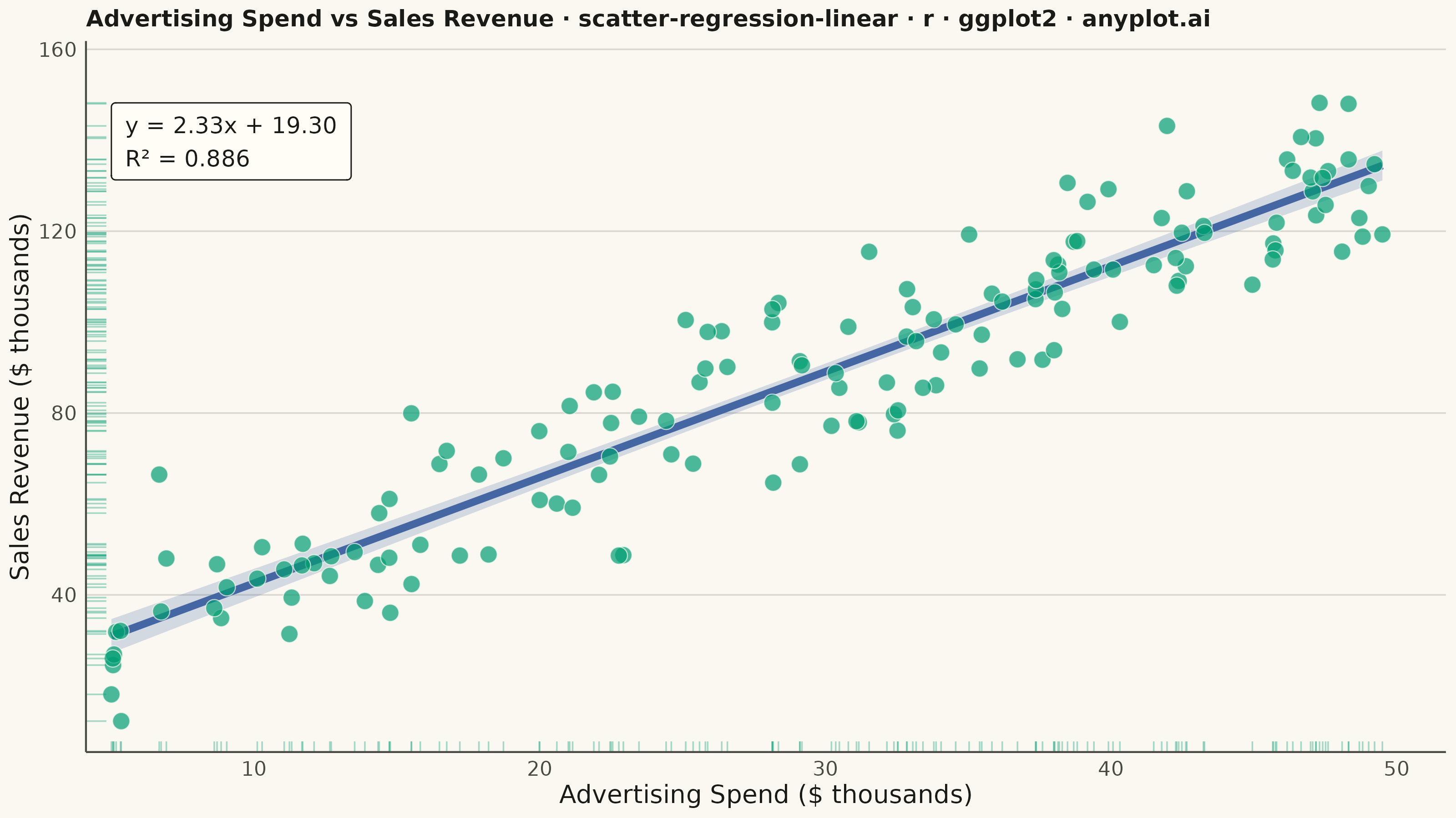
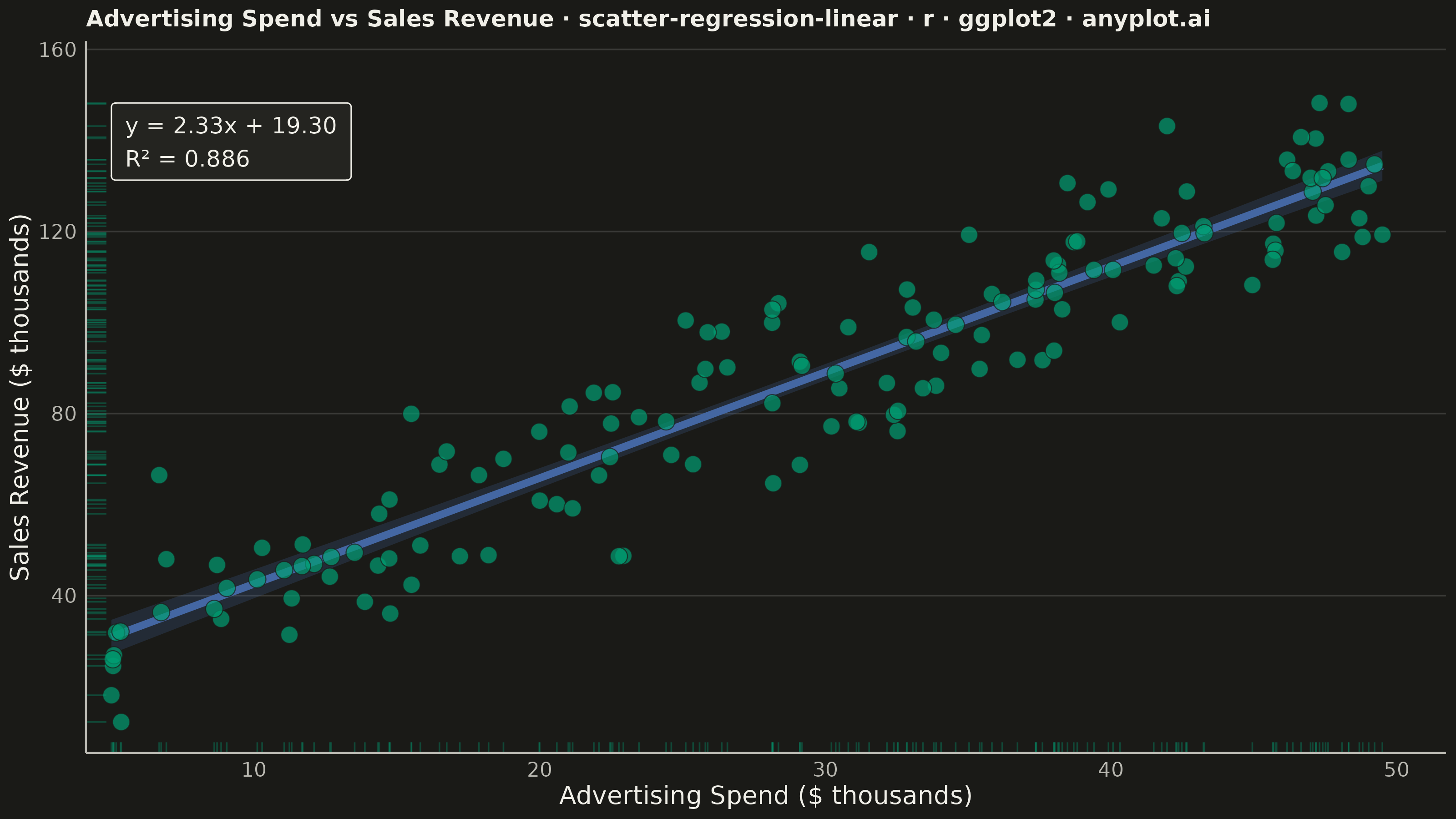
A scatter plot that displays the relationship between two numeric variables with a fitted linear regression line and confidence interval band. This visualization extends the basic scatter plot by adding statistical modeling elements, making it ideal for understanding linear relationships, assessing model fit, and communicating the strength of correlations with visual uncertainty quantification.
#' anyplot.ai
#' scatter-regression-linear: Scatter Plot with Linear Regression
#' Library: ggplot2 3.5.1 | R 4.4.1
#' Quality: 91/100 | Created: 2026-08-05

library(ggplot2)
library(ragg)

set.seed(42)

# --- Theme tokens -------------------------------------------------------
THEME       <- Sys.getenv("ANYPLOT_THEME", "light")
PAGE_BG     <- if (THEME == "light") "#FAF8F1" else "#1A1A17"
ELEVATED_BG <- if (THEME == "light") "#FFFDF6" else "#242420"
INK         <- if (THEME == "light") "#1A1A17" else "#F0EFE8"
INK_SOFT    <- if (THEME == "light") "#4A4A44" else "#B8B7B0"
GRID_COLOR  <- grDevices::adjustcolor(INK, alpha.f = 0.15)
IMPRINT_PALETTE <- c("#009E73", "#C475FD", "#4467A3", "#BD8233",
                     "#AE3030", "#2ABCCD", "#954477", "#99B314")

# --- Data -----------------------------------------------------------------
n <- 150
ad_spend <- runif(n, 5, 50)
sales_revenue <- 2.4 * ad_spend + 18 + rnorm(n, 0, 12)
df <- tibble::tibble(ad_spend = ad_spend, sales_revenue = sales_revenue)

fit <- lm(sales_revenue ~ ad_spend, data = df)
slope <- coef(fit)[["ad_spend"]]
intercept <- coef(fit)[["(Intercept)"]]
r_squared <- summary(fit)$r.squared

equation_label <- sprintf("y = %.2fx + %.2f\nR² = %.3f", slope, intercept, r_squared)

# --- Title (fontsize scales with length, see plot-generator.md) -----------
title_text <- paste0(
  "Advertising Spend vs Sales Revenue · scatter-regression-linear · ",
  "r · ggplot2 · anyplot.ai"
)
title_len <- nchar(title_text)
title_size <- if (title_len > 67) round(12 * 67 / title_len) else 12
title_size <- max(title_size, 8)

# --- Plot -------------------------------------------------------------------
p <- ggplot(df, aes(x = ad_spend, y = sales_revenue)) +
  geom_smooth(
    method = "lm", formula = y ~ x, se = TRUE, level = 0.95,
    color = IMPRINT_PALETTE[3], fill = IMPRINT_PALETTE[3],
    linewidth = 1.4, alpha = 0.22
  ) +
  geom_point(
    shape = 21, fill = IMPRINT_PALETTE[1], color = PAGE_BG,
    size = 3, stroke = 0.3, alpha = 0.7
  ) +
  geom_rug(
    sides = "bl", color = IMPRINT_PALETTE[1], alpha = 0.35,
    linewidth = 0.3, length = unit(0.015, "npc")
  ) +
  annotate(
    "label",
    x = min(df$ad_spend), y = max(df$sales_revenue),
    label = equation_label, hjust = 0, vjust = 1,
    size = 3.2, color = INK, fill = ELEVATED_BG, label.size = 0.25,
    label.padding = unit(0.5, "lines")
  ) +
  labs(
    title = title_text,
    x = "Advertising Spend ($ thousands)",
    y = "Sales Revenue ($ thousands)"
  ) +
  scale_x_continuous(expand = expansion(mult = c(0.02, 0.05))) +
  scale_y_continuous(expand = expansion(mult = c(0.05, 0.1))) +
  theme_minimal(base_size = 8) +
  theme(
    plot.background   = element_rect(fill = PAGE_BG, color = PAGE_BG),
    panel.background  = element_rect(fill = PAGE_BG, color = NA),
    panel.grid.major.x = element_blank(),
    panel.grid.major.y = element_line(color = GRID_COLOR, linewidth = 0.3),
    panel.grid.minor  = element_blank(),
    axis.title        = element_text(color = INK, size = 10),
    axis.text         = element_text(color = INK_SOFT, size = 8),
    axis.line         = element_line(color = INK_SOFT),
    plot.title        = element_text(color = INK, size = title_size, face = "bold"),
    panel.border      = element_blank()
  )

# --- Save -------------------------------------------------------------------
ggsave(
  filename = sprintf("plot-%s.png", THEME),
  plot     = p,
  device   = ragg::agg_png,
  width    = 8,
  height   = 4.5,
  units    = "in",
  dpi      = 400
)
Runnable source as JSON, for any HTTP client: https://api.anyplot.ai/specs/scatter-regression-linear/ggplot2/code. Any spec id and library id listed in llms-full.txt fit the same URL shape; every URL below is complete and callable.
{
  "spec_id": "scatter-regression-linear",
  "language": "r",
  "library": "ggplot2",
  "page": "https://anyplot.ai/scatter-regression-linear/r/ggplot2",
  "hub": "https://anyplot.ai/scatter-regression-linear",
  "code_json": "https://api.anyplot.ai/specs/scatter-regression-linear/ggplot2/code",
  "spec_json": "https://api.anyplot.ai/specs/scatter-regression-linear",
  "render_light_png": "https://storage.googleapis.com/anyplot-images/plots/scatter-regression-linear/r/ggplot2/plot-light.png",
  "render_dark_png": "https://storage.googleapis.com/anyplot-images/plots/scatter-regression-linear/r/ggplot2/plot-dark.png",
  "quality_score": 91.0,
  "license": "MIT",
  "guide": "https://anyplot.ai/llms.txt"
}
Part of Scatter Plot with Linear Regression on anyplot.ai.