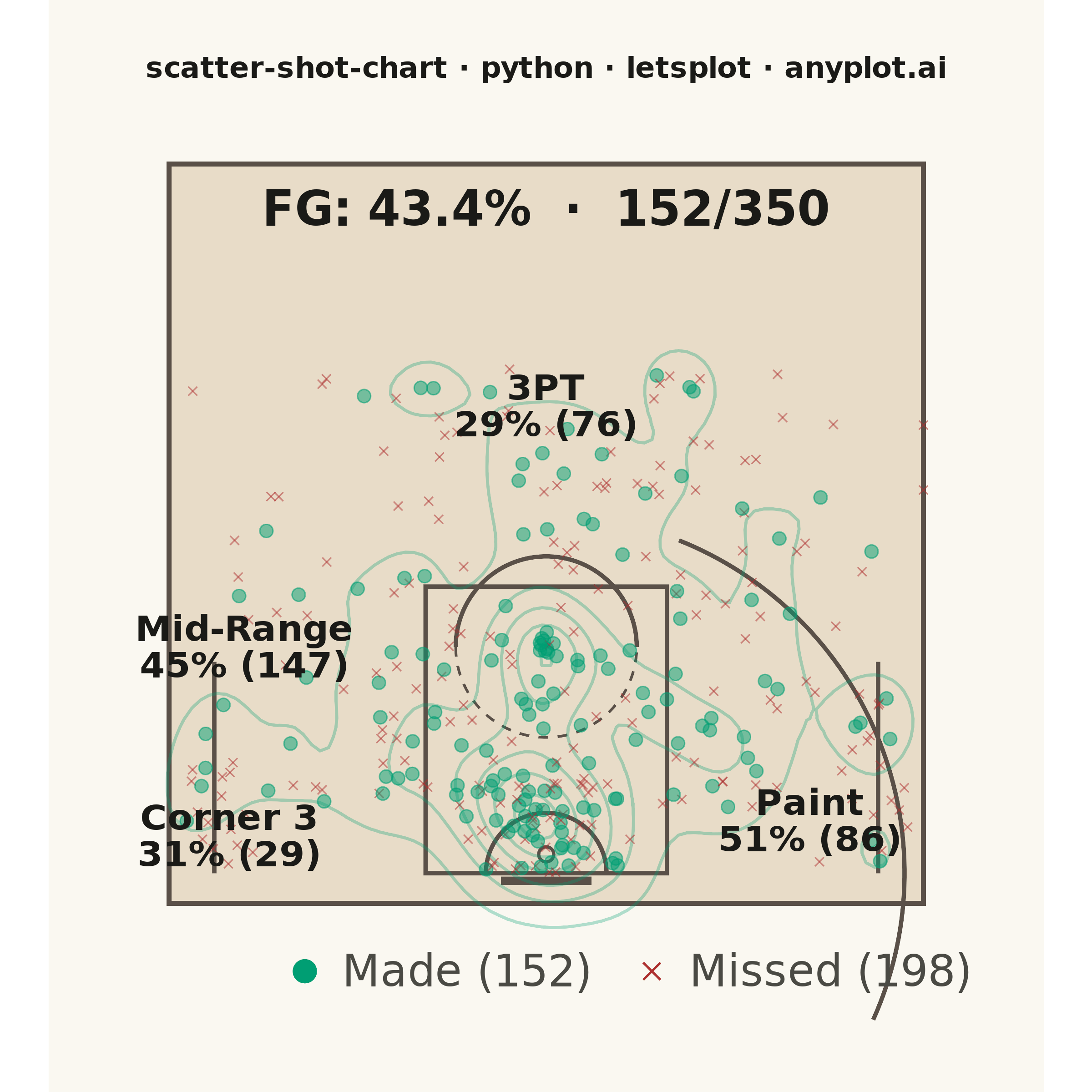
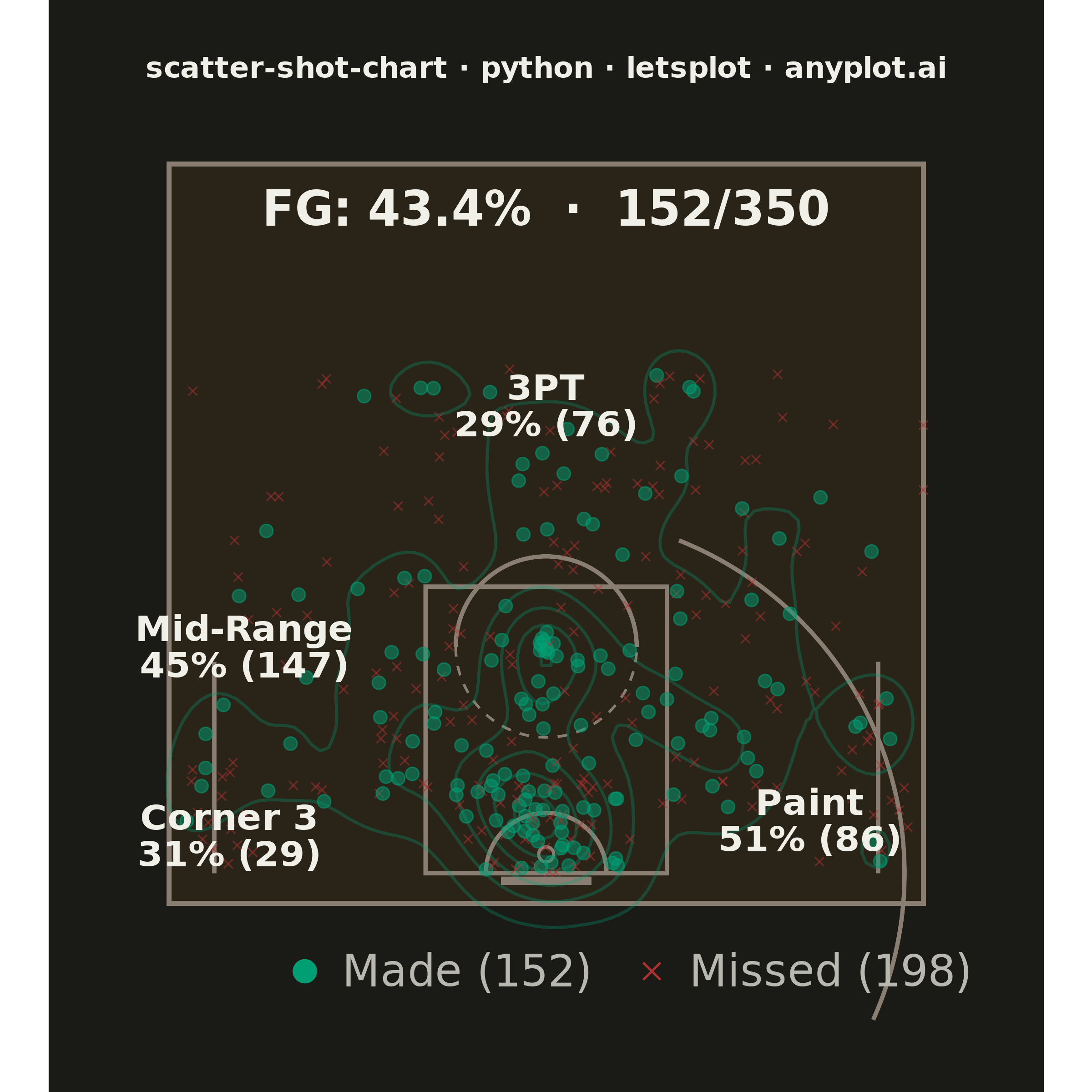
A basketball shot chart overlays shooting data on a half-court diagram, plotting each shot attempt as a point colored by outcome (made or missed). The court drawing includes the three-point arc, free-throw line, paint/key area, and basket, providing spatial context for analyzing shooting patterns and efficiency. Essential for basketball analytics and player evaluation.
""" anyplot.ai
scatter-shot-chart: Basketball Shot Chart
Library: letsplot 4.10.1 | Python 3.13.14
Quality: 90/100 | Updated: 2026-06-21
"""

import os

import numpy as np
import pandas as pd
from lets_plot import (
    LetsPlot,
    aes,
    coord_fixed,
    element_rect,
    element_text,
    geom_density2d,
    geom_path,
    geom_point,
    geom_rect,
    geom_segment,
    geom_text,
    ggplot,
    ggsave,
    ggsize,
    labs,
    layer_tooltips,
    scale_alpha_identity,
    scale_color_identity,
    scale_fill_identity,
    scale_shape_identity,
    scale_size_identity,
    theme,
    theme_void,
    xlim,
    ylim,
)


LetsPlot.setup_html()

# Theme tokens
THEME = os.getenv("ANYPLOT_THEME", "light")
PAGE_BG = "#FAF8F1" if THEME == "light" else "#1A1A17"
ELEVATED_BG = "#FFFDF6" if THEME == "light" else "#242420"
INK = "#1A1A17" if THEME == "light" else "#F0EFE8"
INK_SOFT = "#4A4A44" if THEME == "light" else "#B8B7B0"
INK_MUTED = "#6B6A63" if THEME == "light" else "#A8A79F"

# Imprint palette — semantic assignments
MADE_COLOR = "#009E73"  # Imprint position 1: green = made (good outcome)
MISSED_COLOR = "#AE3030"  # Imprint semantic anchor: red = missed (bad/loss)

# Court visual tokens (domain element — warm hardwood tone, theme-variant)
COURT_COLOR = "#E8DCC8" if THEME == "light" else "#2A2318"
LINE_COLOR = "#5A5048" if THEME == "light" else "#8A7E72"
ANNOTATION_BG = "rgba(232,220,200,0.85)" if THEME == "light" else "rgba(42,35,24,0.88)"

# Data
np.random.seed(42)

n_shots = 350
shot_x = np.concatenate(
    [
        np.random.normal(0, 3, 80),  # paint area
        np.random.normal(0, 7, 60),  # mid-range center
        np.random.normal(-12, 4, 25),  # mid-range left
        np.random.normal(12, 4, 25),  # mid-range right
        np.random.uniform(-22, 22, 60),  # above-break 3
        np.random.normal(-22, 1.2, 20),  # left corner 3
        np.random.normal(22, 1.2, 20),  # right corner 3
        np.random.normal(0, 12, 50),  # deep 3
        np.random.normal(0, 0.5, 10),  # free throws
    ]
)
shot_y = np.concatenate(
    [
        np.random.uniform(0, 6, 80),  # paint area
        np.random.uniform(6, 16, 60),  # mid-range center
        np.random.uniform(4, 14, 25),  # mid-range left
        np.random.uniform(4, 14, 25),  # mid-range right
        np.random.uniform(16, 26, 60),  # above-break 3
        np.random.uniform(0, 12, 20),  # left corner 3
        np.random.uniform(0, 12, 20),  # right corner 3
        np.random.uniform(24, 34, 50),  # deep 3
        np.random.normal(15, 0.3, 10),  # free throws
    ]
)

shot_x = np.clip(shot_x, -25, 25)
shot_y = np.clip(shot_y, 0, 40)

three_pt_dist = np.sqrt(shot_x**2 + shot_y**2)
is_corner_three = (np.abs(shot_x) > 21) & (shot_y < 14)
is_three = (three_pt_dist > 23.75) | is_corner_three
is_free_throw = (np.abs(shot_x) < 1) & (np.abs(shot_y - 15) < 1)

shot_type = np.where(is_free_throw, "free-throw", np.where(is_three, "3-pointer", "2-pointer"))

base_pct = np.where(shot_type == "free-throw", 0.78, np.where(shot_type == "2-pointer", 0.50, 0.35))
dist = np.sqrt(shot_x**2 + shot_y**2)
fg_pct = np.clip(base_pct - dist * 0.004, 0.15, 0.85)
made = np.random.random(n_shots) < fg_pct

zone = np.full(n_shots, "Mid-Range", dtype=object)
zone[dist < 8] = "Paint"
zone[is_three & ~is_corner_three] = "Above Break 3"
zone[is_corner_three] = "Corner 3"
zone[is_free_throw] = "Free Throw"

df = pd.DataFrame(
    {
        "x": shot_x,
        "y": shot_y,
        "made": made,
        "shot_type": shot_type,
        "zone": zone,
        "result": np.where(made, "Made", "Missed"),
        "color": np.where(made, MADE_COLOR, MISSED_COLOR),
        "fill": np.where(made, MADE_COLOR, MISSED_COLOR),
        "point_size": np.where(made, 3.0, 2.5),
        "point_shape": np.where(made, 21, 4),  # circle vs X
    }
)

zone_stats = {}
for z in ["Paint", "Mid-Range", "Above Break 3", "Corner 3"]:
    mask = zone == z
    if mask.sum() > 0:
        zone_stats[z] = (made[mask].sum() / mask.sum() * 100, int(mask.sum()))

# Court geometry (NBA half-court: 50 ft wide x 47 ft deep)
theta_3pt = np.linspace(-np.pi / 2 + 0.38, np.pi / 2 - 0.38, 100)
df_three_arc = pd.DataFrame({"x": 23.75 * np.cos(theta_3pt), "y": 23.75 * np.sin(theta_3pt)})

theta_ft_upper = np.linspace(0, np.pi, 60)
df_ft_arc = pd.DataFrame({"x": 6 * np.cos(theta_ft_upper), "y": 15 + 6 * np.sin(theta_ft_upper)})
theta_ft_lower = np.linspace(np.pi, 2 * np.pi, 60)
df_ft_dash = pd.DataFrame({"x": 6 * np.cos(theta_ft_lower), "y": 15 + 6 * np.sin(theta_ft_lower)})

theta_ra = np.linspace(0, np.pi, 40)
df_restricted = pd.DataFrame({"x": 4 * np.cos(theta_ra), "y": 4 * np.sin(theta_ra)})

n_made = int(made.sum())
n_missed = int((~made).sum())
fg_percent = n_made / n_shots * 100

# Zone annotation positions — four quadrants to avoid overlapping shot clusters
zone_annotations = pd.DataFrame(
    {
        "x": [17.5, -20.0, 0.0, -21.0],
        "y": [3.5, 15.0, 31.0, 2.5],
        "label": [
            f"Paint\n{zone_stats['Paint'][0]:.0f}% ({zone_stats['Paint'][1]})",
            f"Mid-Range\n{zone_stats['Mid-Range'][0]:.0f}% ({zone_stats['Mid-Range'][1]})",
            f"3PT\n{zone_stats['Above Break 3'][0]:.0f}% ({zone_stats['Above Break 3'][1]})",
            f"Corner 3\n{zone_stats['Corner 3'][0]:.0f}% ({zone_stats['Corner 3'][1]})",
        ],
    }
)

# Manual legend at the bottom — wide spacing for clarity
legend_y = -6.5
df_legend = pd.DataFrame(
    {
        "x": [-16.0, 7.0],
        "y": [legend_y, legend_y],
        "color": [MADE_COLOR, MISSED_COLOR],
        "fill": [MADE_COLOR, MISSED_COLOR],
        "shape": [21, 4],
    }
)
df_legend_text = pd.DataFrame(
    {"x": [-13.5, 9.5], "y": [legend_y, legend_y], "label": [f"Made ({n_made})", f"Missed ({n_missed})"]}
)

df_made = df[df["made"]].copy()

# Title — 51 chars, under 67-char baseline so base_size=16 is fine
title = "scatter-shot-chart · python · letsplot · anyplot.ai"
title_len = len(title)
title_size = round(16 * 67 / title_len) if title_len > 67 else 16

# Plot
plot = (
    ggplot()
    # Outer background (page surface)
    + geom_rect(
        aes(xmin="xmin", ymin="ymin", xmax="xmax", ymax="ymax"),
        data=pd.DataFrame({"xmin": [-28], "ymin": [-10], "xmax": [28], "ymax": [49]}),
        fill=PAGE_BG,
        color=PAGE_BG,
    )
    # Court surface
    + geom_rect(
        aes(xmin="xmin", ymin="ymin", xmax="xmax", ymax="ymax"),
        data=pd.DataFrame({"xmin": [-25], "ymin": [-2], "xmax": [25], "ymax": [47]}),
        fill=COURT_COLOR,
        color=LINE_COLOR,
        size=1.2,
    )
    # Paint / key area
    + geom_rect(
        aes(xmin="xmin", ymin="ymin", xmax="xmax", ymax="ymax"),
        data=pd.DataFrame({"xmin": [-8], "ymin": [0], "xmax": [8], "ymax": [19]}),
        fill="rgba(0,0,0,0)",
        color=LINE_COLOR,
        size=1.0,
    )
    # Corner three-point sidelines
    + geom_segment(
        aes(x="x", y="y", xend="xend", yend="yend"),
        data=pd.DataFrame({"x": [-22, 22], "y": [0, 0], "xend": [-22, 22], "yend": [14, 14]}),
        color=LINE_COLOR,
        size=1.0,
    )
    # Three-point arc
    + geom_path(data=df_three_arc, mapping=aes(x="x", y="y"), color=LINE_COLOR, size=1.0)
    # Free-throw circle (solid top, dashed bottom)
    + geom_path(data=df_ft_arc, mapping=aes(x="x", y="y"), color=LINE_COLOR, size=1.0)
    + geom_path(data=df_ft_dash, mapping=aes(x="x", y="y"), color=LINE_COLOR, size=0.6, linetype="dashed")
    # Restricted area arc
    + geom_path(data=df_restricted, mapping=aes(x="x", y="y"), color=LINE_COLOR, size=1.0)
    # Backboard
    + geom_segment(
        aes(x="x", y="y", xend="xend", yend="yend"),
        data=pd.DataFrame({"x": [-3], "y": [-0.5], "xend": [3], "yend": [-0.5]}),
        color=LINE_COLOR,
        size=2.0,
    )
    # Rim
    + geom_point(aes(x="x", y="y"), data=pd.DataFrame({"x": [0], "y": [1.25]}), color=LINE_COLOR, size=3, shape=1)
    # Density contours for made shots — distinctive lets-plot feature showing hot zones
    + geom_density2d(
        data=df_made, mapping=aes(x="x", y="y"), color=MADE_COLOR, alpha=0.3, size=0.7, bins=6, show_legend=False
    )
    # Shot data with lets-plot interactive tooltips
    + geom_point(
        data=df,
        mapping=aes(x="x", y="y", color="color", fill="fill", size="point_size", shape="point_shape"),
        stroke=0.3,
        alpha=0.5,
        tooltips=layer_tooltips()
        .line("@result | @shot_type")
        .line("Zone: @zone")
        .format("x", ".1f")
        .format("y", ".1f")
        .line("Position: (@x, @y)"),
    )
    # Zone FG% annotations — positioned in sparse court areas to minimize overlap
    + geom_text(
        data=zone_annotations,
        mapping=aes(x="x", y="y", label="label"),
        size=10,
        color=INK,
        fontface="bold",
        label_padding=0.4,
        fill=ANNOTATION_BG,
        label_size=0,
    )
    # Overall FG% summary
    + geom_text(
        data=pd.DataFrame({"x": [0], "y": [44], "label": [f"FG: {fg_percent:.1f}%  ·  {n_made}/{n_shots}"]}),
        mapping=aes(x="x", y="y", label="label"),
        size=13,
        color=INK,
        fontface="bold",
    )
    # Legend markers
    + geom_point(aes(x="x", y="y", color="color", fill="fill", shape="shape"), data=df_legend, size=5, stroke=0.5)
    # Legend labels
    + geom_text(data=df_legend_text, mapping=aes(x="x", y="y", label="label"), size=12, color=INK_SOFT, hjust=0)
    + scale_color_identity()
    + scale_fill_identity()
    + scale_size_identity()
    + scale_shape_identity()
    + scale_alpha_identity()
    + coord_fixed(ratio=1)
    + xlim(-28, 28)
    + ylim(-10, 49)
    + labs(title=title)
    + theme_void()
    + theme(
        plot_title=element_text(size=title_size, hjust=0.5, color=INK, face="bold"),
        plot_background=element_rect(fill=PAGE_BG, color=PAGE_BG),
        plot_margin=[30, 15, 10, 15],
    )
    + ggsize(600, 600)
)

# Save — square canvas: ggsize(600, 600) × scale=4 → 2400×2400 px
ggsave(plot, f"plot-{THEME}.png", path=".", scale=4)
ggsave(plot, f"plot-{THEME}.html", path=".")
Runnable source as JSON, for any HTTP client: https://api.anyplot.ai/specs/scatter-shot-chart/letsplot/code. Any spec id and library id listed in llms-full.txt fit the same URL shape; every URL below is complete and callable.
{
  "spec_id": "scatter-shot-chart",
  "language": "python",
  "library": "letsplot",
  "page": "https://anyplot.ai/scatter-shot-chart/python/letsplot",
  "hub": "https://anyplot.ai/scatter-shot-chart",
  "code_json": "https://api.anyplot.ai/specs/scatter-shot-chart/letsplot/code",
  "spec_json": "https://api.anyplot.ai/specs/scatter-shot-chart",
  "render_light_png": "https://storage.googleapis.com/anyplot-images/plots/scatter-shot-chart/python/letsplot/plot-light.png",
  "render_dark_png": "https://storage.googleapis.com/anyplot-images/plots/scatter-shot-chart/python/letsplot/plot-dark.png",
  "interactive_light_html": "https://storage.googleapis.com/anyplot-images/plots/scatter-shot-chart/python/letsplot/plot-light.html",
  "interactive_dark_html": "https://storage.googleapis.com/anyplot-images/plots/scatter-shot-chart/python/letsplot/plot-dark.html",
  "quality_score": 90.0,
  "license": "MIT",
  "guide": "https://anyplot.ai/llms.txt"
}
Part of Basketball Shot Chart on anyplot.ai.