The same plot in 14 other libraries — Python: Altair, Bokeh, lets-plot, Matplotlib, Plotly, Pygal, Seaborn; R: ggplot2; Julia: Makie.jl; JavaScript: Chart.js, D3.js, Apache ECharts, Highcharts, MUI X Charts. Compare all 15 side by side: Basketball Shot Chart in Python, R, Julia and JavaScript.
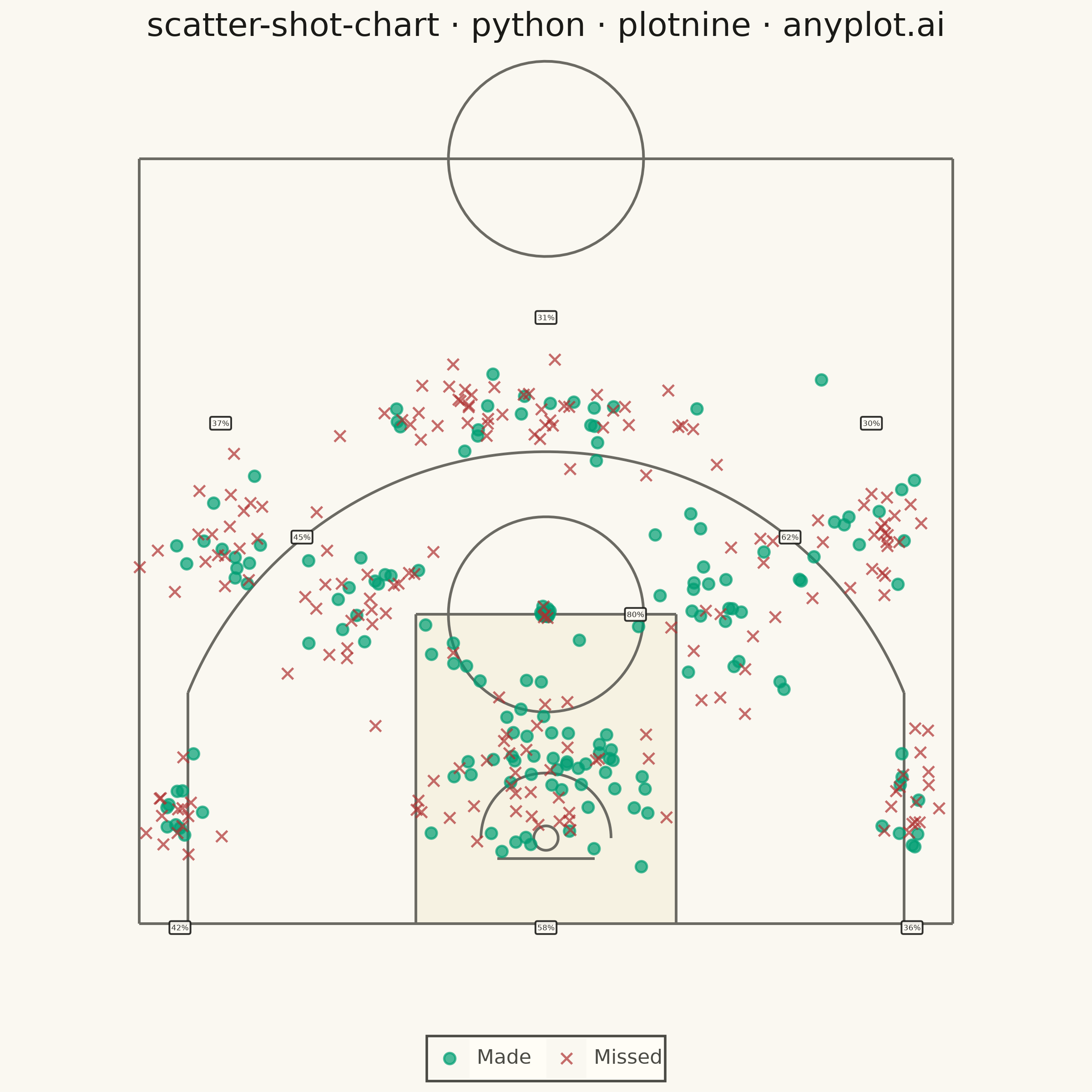
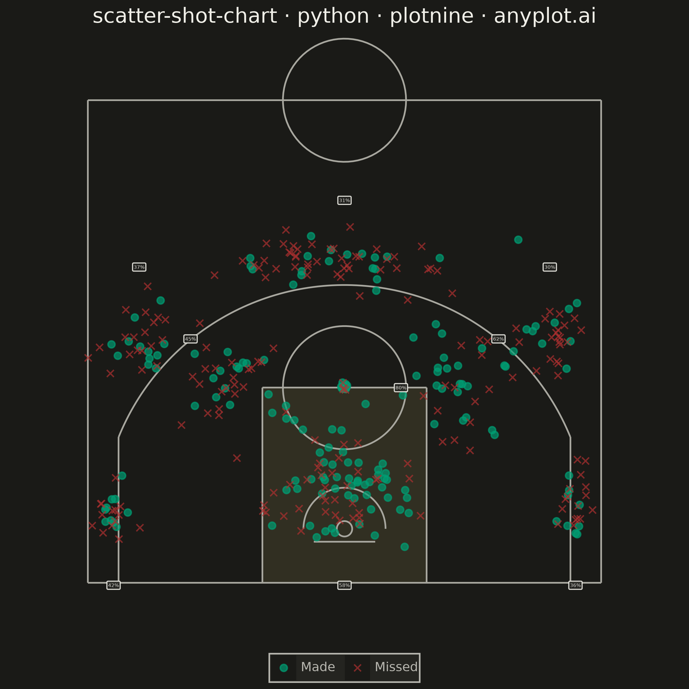
A basketball shot chart overlays shooting data on a half-court diagram, plotting each shot attempt as a point colored by outcome (made or missed). The court drawing includes the three-point arc, free-throw line, paint/key area, and basket, providing spatial context for analyzing shooting patterns and efficiency. Essential for basketball analytics and player evaluation.
""" anyplot.ai
scatter-shot-chart: Basketball Shot Chart
Library: plotnine 0.15.7 | Python 3.13.14
Quality: 84/100 | Created: 2026-06-21
"""

import os
import sys


# Prevent self-import: when Python runs plotnine.py its own directory lands on
# sys.path[0], shadowing the real plotnine library.  Remove it before the import.
_this_dir = os.path.dirname(os.path.abspath(__file__))
sys.path = [p for p in sys.path if os.path.abspath(p or ".") != _this_dir]

import numpy as np
import pandas as pd
from plotnine import (
    aes,
    coord_fixed,
    element_blank,
    element_rect,
    element_text,
    geom_label,
    geom_path,
    geom_point,
    geom_rect,
    ggplot,
    labs,
    scale_color_manual,
    scale_shape_manual,
    theme,
)


# Theme tokens
THEME = os.getenv("ANYPLOT_THEME", "light")
PAGE_BG = "#FAF8F1" if THEME == "light" else "#1A1A17"
ELEVATED_BG = "#FFFDF6" if THEME == "light" else "#242420"
INK = "#1A1A17" if THEME == "light" else "#F0EFE8"
INK_SOFT = "#4A4A44" if THEME == "light" else "#B8B7B0"
INK_MUTED = "#6B6A63" if THEME == "light" else "#A8A79F"

# Imprint palette — semantic assignment
MADE_COLOR = "#009E73"  # brand green (made = success)
MISSED_COLOR = "#AE3030"  # matte red (miss = failure)
COURT_COLOR = INK_MUTED
PAINT_FILL = "#DDCC77"  # Imprint amber — subtle hardwood zone tint

# NBA half-court dimensions (feet, basket center at origin)
BASELINE_Y = -5.25  # baseline is 5.25 ft behind basket rim
HALFCOURT_Y = 41.75  # half-court line from basket
THREE_R = 23.75  # three-point arc radius
CORNER_X = 22.0  # x where corner three meets the arc
CORNER_BREAK_Y = float(np.sqrt(THREE_R**2 - CORNER_X**2))  # ~8.95 ft
FT_Y = 13.75  # free-throw line distance from basket
FT_R = 6.0  # free-throw circle radius
PAINT_W = 8.0  # half-width of the 16 ft key/paint
BACKBOARD_Y = -1.25  # backboard (4 ft from baseline)

# Court geometry — one DataFrame per segment, combined for geom_path
_segs = []

# Outer boundary
_segs.append(pd.DataFrame({"x": [-25, 25], "y": [BASELINE_Y] * 2, "seg": "baseline"}))
_segs.append(pd.DataFrame({"x": [25] * 2, "y": [BASELINE_Y, HALFCOURT_Y], "seg": "side_r"}))
_segs.append(pd.DataFrame({"x": [-25] * 2, "y": [BASELINE_Y, HALFCOURT_Y], "seg": "side_l"}))
_segs.append(pd.DataFrame({"x": [-25, 25], "y": [HALFCOURT_Y] * 2, "seg": "halfcourt"}))

# Paint / key rectangle
_segs.append(pd.DataFrame({"x": [-PAINT_W] * 2, "y": [BASELINE_Y, FT_Y], "seg": "paint_l"}))
_segs.append(pd.DataFrame({"x": [PAINT_W] * 2, "y": [BASELINE_Y, FT_Y], "seg": "paint_r"}))
_segs.append(pd.DataFrame({"x": [-PAINT_W, PAINT_W], "y": [FT_Y] * 2, "seg": "ft_line"}))

# Free-throw circle upper half
_a = np.linspace(0, np.pi, 60)
_segs.append(pd.DataFrame({"x": FT_R * np.cos(_a), "y": FT_Y + FT_R * np.sin(_a), "seg": "ft_upper"}))

# Free-throw circle lower half (dashed in real life — drawn here for context)
_a = np.linspace(np.pi, 2 * np.pi, 60)
_segs.append(pd.DataFrame({"x": FT_R * np.cos(_a), "y": FT_Y + FT_R * np.sin(_a), "seg": "ft_lower"}))

# Three-point arc (right corner break to left, sweeping through top)
_theta1 = float(np.arctan2(CORNER_BREAK_Y, CORNER_X))
_theta2 = np.pi - _theta1
_a = np.linspace(_theta1, _theta2, 120)
_segs.append(pd.DataFrame({"x": THREE_R * np.cos(_a), "y": THREE_R * np.sin(_a), "seg": "three_arc"}))

# Corner three straight sections
_segs.append(pd.DataFrame({"x": [CORNER_X] * 2, "y": [BASELINE_Y, CORNER_BREAK_Y], "seg": "corner_r"}))
_segs.append(pd.DataFrame({"x": [-CORNER_X] * 2, "y": [BASELINE_Y, CORNER_BREAK_Y], "seg": "corner_l"}))

# Restricted area arc (4 ft radius)
_a = np.linspace(0, np.pi, 60)
_segs.append(pd.DataFrame({"x": 4.0 * np.cos(_a), "y": 4.0 * np.sin(_a), "seg": "restricted"}))

# Basket rim circle (0.75 ft radius)
_a = np.linspace(0, 2 * np.pi, 60)
_segs.append(pd.DataFrame({"x": 0.75 * np.cos(_a), "y": 0.75 * np.sin(_a), "seg": "basket"}))

# Backboard
_segs.append(pd.DataFrame({"x": [-3.0, 3.0], "y": [BACKBOARD_Y] * 2, "seg": "backboard"}))

# Half-court center circle (6 ft radius — partially visible at top)
_a = np.linspace(0, 2 * np.pi, 80)
_segs.append(pd.DataFrame({"x": 6.0 * np.cos(_a), "y": HALFCOURT_Y + 6.0 * np.sin(_a), "seg": "hc_circle"}))

court_df = pd.concat(_segs, ignore_index=True)

# Paint area tint for zone context
paint_rect = pd.DataFrame({"xmin": [-PAINT_W], "xmax": [PAINT_W], "ymin": [BASELINE_Y], "ymax": [FT_Y]})

# Shot data — simulated NBA player shot chart with shot_type field
np.random.seed(42)

_zone_specs = [
    # (x_center, y_center, x_std, y_std, n, fg_pct, shot_type, zone_key)
    (0, 4.0, 4.0, 3.0, 90, 0.62, "2-pointer", "paint"),
    (-11, FT_Y, 2.5, 3.0, 40, 0.41, "2-pointer", "l_elbow"),
    (11, FT_Y, 2.5, 3.0, 40, 0.41, "2-pointer", "r_elbow"),
    (0, 26.0, 5.5, 1.5, 65, 0.37, "3-pointer", "top3"),
    (-22.5, 2.0, 1.0, 1.8, 25, 0.42, "3-pointer", "l_corner"),
    (22.5, 2.0, 1.0, 1.8, 25, 0.42, "3-pointer", "r_corner"),
    (-20, 19, 2.0, 2.0, 30, 0.34, "3-pointer", "l_wing"),
    (20, 19, 2.0, 2.0, 30, 0.34, "3-pointer", "r_wing"),
    (0.0, FT_Y, 0.2, 0.2, 20, 0.78, "free-throw", "ft"),
]

_all_x, _all_y, _all_m, _all_type, _all_zone = [], [], [], [], []
for _xc, _yc, _xs, _ys, _n, _fg, _stype, _zkey in _zone_specs:
    _x = np.random.normal(_xc, _xs, _n)
    _y = np.random.normal(_yc, _ys, _n)
    _m = np.random.random(_n) < _fg
    _all_x.extend(_x)
    _all_y.extend(_y)
    _all_m.extend(_m)
    _all_type.extend([_stype] * _n)
    _all_zone.extend([_zkey] * _n)

shots_df = pd.DataFrame({"x": _all_x, "y": _all_y, "made": _all_m, "shot_type": _all_type, "zone": _all_zone})
shots_df["outcome"] = shots_df["made"].map({True: "Made", False: "Missed"})
shots_df = shots_df[shots_df["x"].between(-25, 25) & shots_df["y"].between(BASELINE_Y, HALFCOURT_Y)].reset_index(
    drop=True
)

# Per-zone FG% annotations — computed from actual data
_zone_fg = shots_df.groupby("zone")["made"].mean()

_zone_annot_pos = {
    "paint": (0.0, -5.5),
    "l_elbow": (-15.0, 18.5),
    "r_elbow": (15.0, 18.5),
    "top3": (0.0, 32.0),
    "l_corner": (-22.5, -5.5),
    "r_corner": (22.5, -5.5),
    "l_wing": (-20.0, 25.5),
    "r_wing": (20.0, 25.5),
    "ft": (5.5, FT_Y),
}

annot_df = pd.DataFrame(
    [
        {"x": ax, "y": ay, "label": f"{_zone_fg[zkey]:.0%}"}
        for zkey, (ax, ay) in _zone_annot_pos.items()
        if zkey in _zone_fg.index
    ]
)

# Plot — square canvas for 1:1 court geometry (2400×2400 at dpi=400)
_title = "scatter-shot-chart · python · plotnine · anyplot.ai"

plot = (
    ggplot()
    # Paint zone tint — subtle amber for hardwood spatial context
    + geom_rect(
        data=paint_rect,
        mapping=aes(xmin="xmin", xmax="xmax", ymin="ymin", ymax="ymax"),
        fill=PAINT_FILL,
        color="none",
        alpha=0.12,
    )
    # Court lines
    + geom_path(data=court_df, mapping=aes(x="x", y="y", group="seg"), color=COURT_COLOR, size=0.6)
    # Shot markers — color + shape redundant encoding for CVD accessibility
    + geom_point(data=shots_df, mapping=aes(x="x", y="y", color="outcome", shape="outcome"), size=2.0, alpha=0.70)
    + scale_color_manual(values={"Made": MADE_COLOR, "Missed": MISSED_COLOR}, name="")
    + scale_shape_manual(values={"Made": "o", "Missed": "x"}, name="")
    # Per-zone FG% callouts via geom_label (plotnine-native background fill)
    + geom_label(
        data=annot_df,
        mapping=aes(x="x", y="y", label="label"),
        color=INK,
        fill=ELEVATED_BG,
        size=3.0,
        ha="center",
        va="center",
        alpha=0.90,
    )
    + coord_fixed(ratio=1, xlim=(-26.5, 26.5), ylim=(-7.5, 45.5))
    + labs(title=_title, x="", y="")
    + theme(
        figure_size=(6, 6),
        plot_background=element_rect(fill=PAGE_BG, color=PAGE_BG),
        panel_background=element_rect(fill=PAGE_BG),
        panel_grid_major=element_blank(),
        panel_grid_minor=element_blank(),
        panel_border=element_blank(),
        axis_title=element_blank(),
        axis_text=element_blank(),
        axis_ticks=element_blank(),
        axis_line=element_blank(),
        plot_title=element_text(color=INK, size=13),
        legend_background=element_rect(fill=ELEVATED_BG, color=INK_SOFT),
        legend_text=element_text(color=INK_SOFT, size=8),
        legend_title=element_blank(),
        legend_key=element_rect(fill=PAGE_BG, color=PAGE_BG),
        legend_position="bottom",
    )
)

plot.save(f"plot-{THEME}.png", dpi=400, width=6, height=6, units="in")
Runnable source as JSON, for any HTTP client: https://api.anyplot.ai/specs/scatter-shot-chart/plotnine/code. Any spec id and library id listed in llms-full.txt fit the same URL shape; every URL below is complete and callable.
{
  "spec_id": "scatter-shot-chart",
  "language": "python",
  "library": "plotnine",
  "page": "https://anyplot.ai/scatter-shot-chart/python/plotnine",
  "hub": "https://anyplot.ai/scatter-shot-chart",
  "code_json": "https://api.anyplot.ai/specs/scatter-shot-chart/plotnine/code",
  "spec_json": "https://api.anyplot.ai/specs/scatter-shot-chart",
  "render_light_png": "https://storage.googleapis.com/anyplot-images/plots/scatter-shot-chart/python/plotnine/plot-light.png",
  "render_dark_png": "https://storage.googleapis.com/anyplot-images/plots/scatter-shot-chart/python/plotnine/plot-dark.png",
  "quality_score": 84.0,
  "license": "MIT",
  "guide": "https://anyplot.ai/llms.txt"
}
Part of Basketball Shot Chart on anyplot.ai.