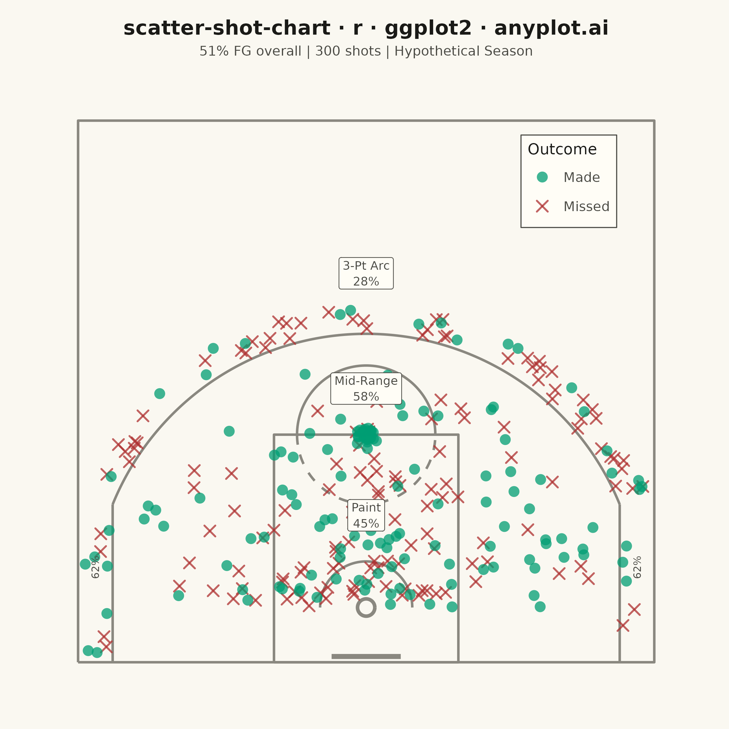
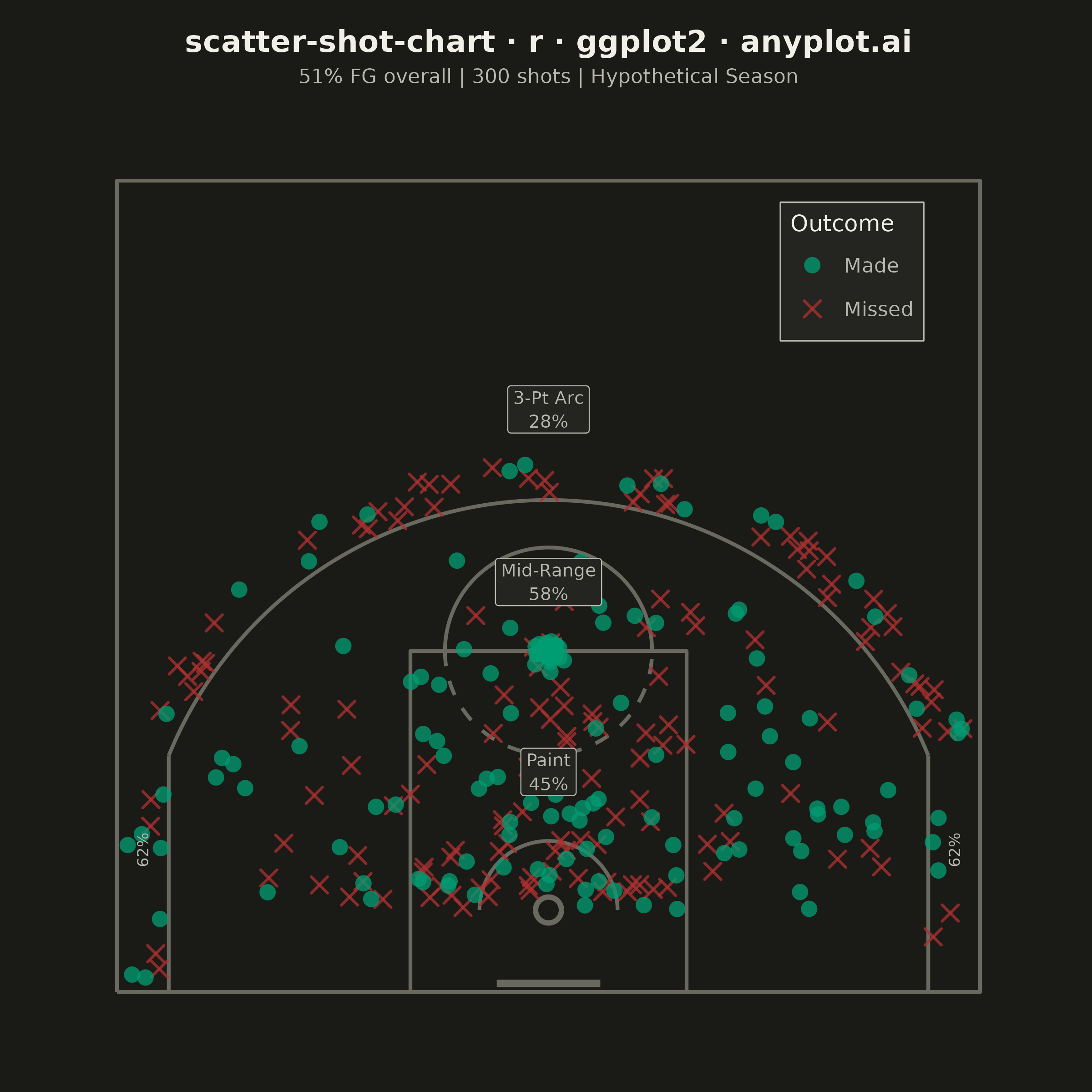
The same plot in 14 other libraries — Python: Altair, Bokeh, lets-plot, Matplotlib, Plotly, plotnine, Pygal, Seaborn; Julia: Makie.jl; JavaScript: Chart.js, D3.js, Apache ECharts, Highcharts, MUI X Charts. Compare all 15 side by side: Basketball Shot Chart in Python, R, Julia and JavaScript.
A basketball shot chart overlays shooting data on a half-court diagram, plotting each shot attempt as a point colored by outcome (made or missed). The court drawing includes the three-point arc, free-throw line, paint/key area, and basket, providing spatial context for analyzing shooting patterns and efficiency. Essential for basketball analytics and player evaluation.
#' anyplot.ai
#' scatter-shot-chart: Basketball Shot Chart
#' Library: ggplot2 3.5.1 | R 4.4.1
#' Quality: 83/100 | Created: 2026-06-21

library(ggplot2)
library(ragg)

set.seed(42)

# Theme tokens (Imprint palette — see prompts/default-style-guide.md)
THEME       <- Sys.getenv("ANYPLOT_THEME", "light")
PAGE_BG     <- if (THEME == "light") "#FAF8F1" else "#1A1A17"
INK         <- if (THEME == "light") "#1A1A17" else "#F0EFE8"
INK_SOFT    <- if (THEME == "light") "#4A4A44" else "#B8B7B0"
ELEVATED_BG <- if (THEME == "light") "#FFFDF6" else "#242420"
COURT_LINE  <- if (THEME == "light") "#8A8880" else "#6A6960"

# Imprint palette — semantic color assignment for shot outcomes
COLOR_MADE   <- "#009E73"  # brand green (position 1) — positive outcome
COLOR_MISSED <- "#AE3030"  # matte red (semantic anchor) — negative outcome

# NBA half-court dimensions in feet (basket center = origin)
BASELINE_Y   <- -4.75
COURT_H      <- 42.25
COURT_W      <- 25.0
THREE_R      <- 23.75
CORNER_X     <- 22.0
CORNER_Y_TOP <- sqrt(THREE_R^2 - CORNER_X^2)  # ~8.95 ft — arc/corner junction
FT_Y         <- 15.0
PAINT_W      <- 8.0
RESTRICT_R   <- 4.0
FT_CIRC_R   <- 6.0
BASKET_R     <- 0.75

# Shot data — 300 attempts from a hypothetical player's season
n_shots   <- 300
shot_type <- sample(c("2-pointer", "3-pointer", "free throw"),
                    n_shots, replace = TRUE, prob = c(0.60, 0.30, 0.10))
n_2pt <- sum(shot_type == "2-pointer")
n_3pt <- sum(shot_type == "3-pointer")
n_ft  <- sum(shot_type == "free throw")

# 2-pointers: distributed inside the three-point arc
ang_2 <- runif(n_2pt, 0, pi)
r_2   <- runif(n_2pt, 1.5, 21.0)
x_2   <- r_2 * cos(ang_2)
y_2   <- r_2 * sin(ang_2)

# 3-pointers: above-the-break and corner variants
arc_alpha <- acos(CORNER_X / THREE_R)
is_corner <- runif(n_3pt) < 0.25
ang_ab    <- runif(n_3pt, arc_alpha, pi - arc_alpha)
r_ab      <- runif(n_3pt, THREE_R + 0.3, THREE_R + 2.5)
x_corn    <- sample(c(-1L, 1L), n_3pt, replace = TRUE) * runif(n_3pt, 22.2, 24.5)
y_corn    <- runif(n_3pt, BASELINE_Y + 0.3, 7.5)
x_3       <- ifelse(is_corner, x_corn, r_ab * cos(ang_ab))
y_3       <- ifelse(is_corner, y_corn, r_ab * sin(ang_ab))

# Free throws: clustered at the free-throw line
x_ft_d <- rnorm(n_ft, 0, 0.4)
y_ft_d <- rnorm(n_ft, FT_Y, 0.4)

# Combine and clip to court bounds
df_shots <- data.frame(
  x    = pmax(-24.5, pmin(24.5, c(x_2, x_3, x_ft_d))),
  y    = pmax(BASELINE_Y + 0.2, pmin(COURT_H - 0.5, c(y_2, y_3, y_ft_d))),
  type = c(rep("2-pointer", n_2pt), rep("3-pointer", n_3pt), rep("free throw", n_ft))
)

# Shot outcomes with realistic field-goal percentages
fg_prob <- ifelse(df_shots$type == "free throw", 0.78,
           ifelse(df_shots$type == "3-pointer",  0.37, 0.47))
df_shots$outcome <- factor(
  ifelse(runif(n_shots) < fg_prob, "Made", "Missed"),
  levels = c("Made", "Missed")
)

# Sort so missed shots render first (bottom layer), made shots on top
df_shots <- df_shots[order(df_shots$outcome, decreasing = TRUE), ]

# Zone classification for efficiency callouts
dist       <- sqrt(df_shots$x^2 + df_shots$y^2)
is_corner3 <- abs(df_shots$x) >= CORNER_X & df_shots$y <= CORNER_Y_TOP
is_3pt     <- dist >= THREE_R | is_corner3
is_paint   <- !is_3pt & abs(df_shots$x) <= PAINT_W & df_shots$y <= FT_Y
df_shots$zone <- ifelse(df_shots$type == "free throw", "ft",
                 ifelse(is_corner3, "corner3",
                 ifelse(is_3pt, "above3",
                 ifelse(is_paint, "paint", "mid"))))

# FG% per zone
zone_fg <- function(zone) {
  s <- df_shots[df_shots$zone == zone, ]
  sprintf("%.0f%%", 100 * mean(s$outcome == "Made"))
}
overall_made <- round(100 * mean(df_shots$outcome == "Made"))
subtitle_str <- sprintf("%d%% FG overall | %d shots | Hypothetical Season",
                        overall_made, n_shots)

# Court geometry data frames
arc_angles <- seq(arc_alpha, pi - arc_alpha, length.out = 200)
df_arc <- data.frame(
  x = THREE_R * cos(arc_angles),
  y = THREE_R * sin(arc_angles)
)
df_ft_top <- data.frame(
  x = FT_CIRC_R * cos(seq(0, pi, length.out = 80)),
  y = FT_Y + FT_CIRC_R * sin(seq(0, pi, length.out = 80))
)
df_ft_bot <- data.frame(
  x = FT_CIRC_R * cos(seq(pi, 2 * pi, length.out = 80)),
  y = FT_Y + FT_CIRC_R * sin(seq(pi, 2 * pi, length.out = 80))
)
df_ra <- data.frame(
  x = RESTRICT_R * cos(seq(0, pi, length.out = 60)),
  y = RESTRICT_R * sin(seq(0, pi, length.out = 60))
)
df_basket <- data.frame(
  x = BASKET_R * cos(seq(0, 2 * pi, length.out = 60)),
  y = BASKET_R * sin(seq(0, 2 * pi, length.out = 60))
)
df_court <- data.frame(
  x = c(-COURT_W, COURT_W, COURT_W, -COURT_W, -COURT_W),
  y = c(BASELINE_Y, BASELINE_Y, COURT_H, COURT_H, BASELINE_Y)
)
df_key <- data.frame(
  x = c(-PAINT_W, PAINT_W, PAINT_W, -PAINT_W, -PAINT_W),
  y = c(BASELINE_Y, BASELINE_Y, FT_Y, FT_Y, BASELINE_Y)
)

# Plot
p <- ggplot() +
  # Court boundary
  geom_path(data = df_court, aes(x, y),
            color = COURT_LINE, linewidth = 0.7) +
  # Paint / key rectangle
  geom_path(data = df_key, aes(x, y),
            color = COURT_LINE, linewidth = 0.7) +
  # Corner three-point lines (straight vertical portions at x = ±22)
  annotate("segment",
           x    = c(-CORNER_X, CORNER_X),
           xend = c(-CORNER_X, CORNER_X),
           y    = c(BASELINE_Y, BASELINE_Y),
           yend = c(CORNER_Y_TOP, CORNER_Y_TOP),
           color = COURT_LINE, linewidth = 0.7) +
  # Three-point arc
  geom_path(data = df_arc, aes(x, y),
            color = COURT_LINE, linewidth = 0.7) +
  # Free-throw circle — solid top half (above key)
  geom_path(data = df_ft_top, aes(x, y),
            color = COURT_LINE, linewidth = 0.7) +
  # Free-throw circle — dashed bottom half (inside key)
  geom_path(data = df_ft_bot, aes(x, y),
            color = COURT_LINE, linewidth = 0.7, linetype = "dashed") +
  # Restricted area arc
  geom_path(data = df_ra, aes(x, y),
            color = COURT_LINE, linewidth = 0.7) +
  # Backboard
  annotate("segment",
           x = -3, xend = 3,
           y = BASELINE_Y + 0.5, yend = BASELINE_Y + 0.5,
           color = COURT_LINE, linewidth = 1.4) +
  # Basket (rim circle)
  geom_path(data = df_basket, aes(x, y),
            color = COURT_LINE, linewidth = 1.0) +
  # Shot attempts — missed drawn first, made on top for visibility
  geom_point(data = df_shots,
             aes(x = x, y = y, color = outcome, shape = outcome),
             size = 2.5, alpha = 0.75, stroke = 0.8) +
  # Color and shape scales (redundant encoding for colorblind accessibility)
  scale_color_manual(
    name   = "Outcome",
    values = c("Made" = COLOR_MADE, "Missed" = COLOR_MISSED)
  ) +
  scale_shape_manual(
    name   = "Outcome",
    values = c("Made" = 16, "Missed" = 4)
  ) +
  # Zone efficiency callouts — FG% per court zone for storytelling (DE-03)
  annotate("label", x = 0, y = 8,
           label = paste0("Paint\n", zone_fg("paint")),
           color = INK_SOFT, fill = ELEVATED_BG, label.size = 0.2,
           size = 2.5, lineheight = 1.1) +
  annotate("label", x = 0, y = 19,
           label = paste0("Mid-Range\n", zone_fg("mid")),
           color = INK_SOFT, fill = ELEVATED_BG, label.size = 0.2,
           size = 2.5, lineheight = 1.1) +
  annotate("label", x = 0, y = 29,
           label = paste0("3-Pt Arc\n", zone_fg("above3")),
           color = INK_SOFT, fill = ELEVATED_BG, label.size = 0.2,
           size = 2.5, lineheight = 1.1) +
  annotate("text", x = -23.5, y = 3.5, label = zone_fg("corner3"),
           color = INK_SOFT, size = 2.2, angle = 90) +
  annotate("text", x = 23.5, y = 3.5, label = zone_fg("corner3"),
           color = INK_SOFT, size = 2.2, angle = 90) +
  # 1:1 aspect ratio — court must not be distorted
  coord_fixed(ratio = 1, xlim = c(-26, 26), ylim = c(-6, 44)) +
  labs(
    title    = "scatter-shot-chart · r · ggplot2 · anyplot.ai",
    subtitle = subtitle_str
  ) +
  theme_minimal(base_size = 8) +
  theme(
    plot.background   = element_rect(fill = PAGE_BG, color = PAGE_BG),
    panel.background  = element_rect(fill = PAGE_BG, color = NA),
    panel.grid        = element_blank(),
    panel.border      = element_blank(),
    axis.title        = element_blank(),
    axis.text         = element_blank(),
    axis.ticks        = element_blank(),
    plot.title        = element_text(color = INK, size = 12, hjust = 0.5,
                                     face = "bold", margin = margin(b = 4)),
    plot.subtitle     = element_text(color = INK_SOFT, size = 8, hjust = 0.5,
                                     margin = margin(b = 8)),
    legend.background = element_rect(fill = ELEVATED_BG, color = INK_SOFT,
                                     linewidth = 0.3),
    legend.text       = element_text(color = INK_SOFT, size = 8),
    legend.title      = element_text(color = INK, size = 9),
    legend.position          = "inside",
    legend.position.inside   = c(0.88, 0.90),
    legend.justification.inside = c(1, 1),
    plot.margin       = margin(12, 12, 12, 12, "pt")
  )

# Save — square canvas (2400×2400 px) for undistorted court geometry
ggsave(
  filename = sprintf("plot-%s.png", THEME),
  plot     = p,
  device   = ragg::agg_png,
  width    = 6,
  height   = 6,
  units    = "in",
  dpi      = 400
)
Runnable source as JSON, for any HTTP client: https://api.anyplot.ai/specs/scatter-shot-chart/ggplot2/code. Any spec id and library id listed in llms-full.txt fit the same URL shape; every URL below is complete and callable.
{
  "spec_id": "scatter-shot-chart",
  "language": "r",
  "library": "ggplot2",
  "page": "https://anyplot.ai/scatter-shot-chart/r/ggplot2",
  "hub": "https://anyplot.ai/scatter-shot-chart",
  "code_json": "https://api.anyplot.ai/specs/scatter-shot-chart/ggplot2/code",
  "spec_json": "https://api.anyplot.ai/specs/scatter-shot-chart",
  "render_light_png": "https://storage.googleapis.com/anyplot-images/plots/scatter-shot-chart/r/ggplot2/plot-light.png",
  "render_dark_png": "https://storage.googleapis.com/anyplot-images/plots/scatter-shot-chart/r/ggplot2/plot-dark.png",
  "quality_score": 83.0,
  "license": "MIT",
  "guide": "https://anyplot.ai/llms.txt"
}
Part of Basketball Shot Chart on anyplot.ai.