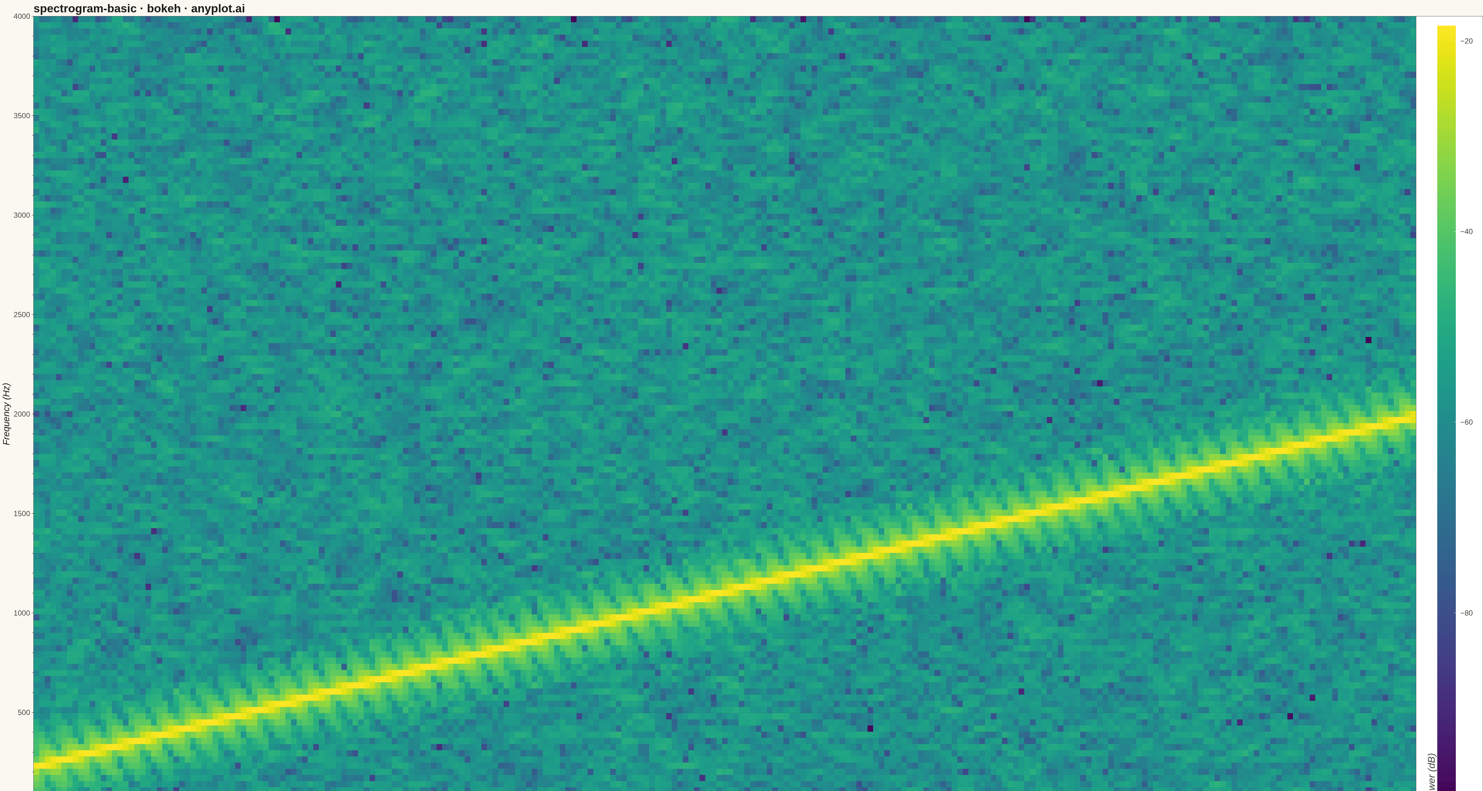
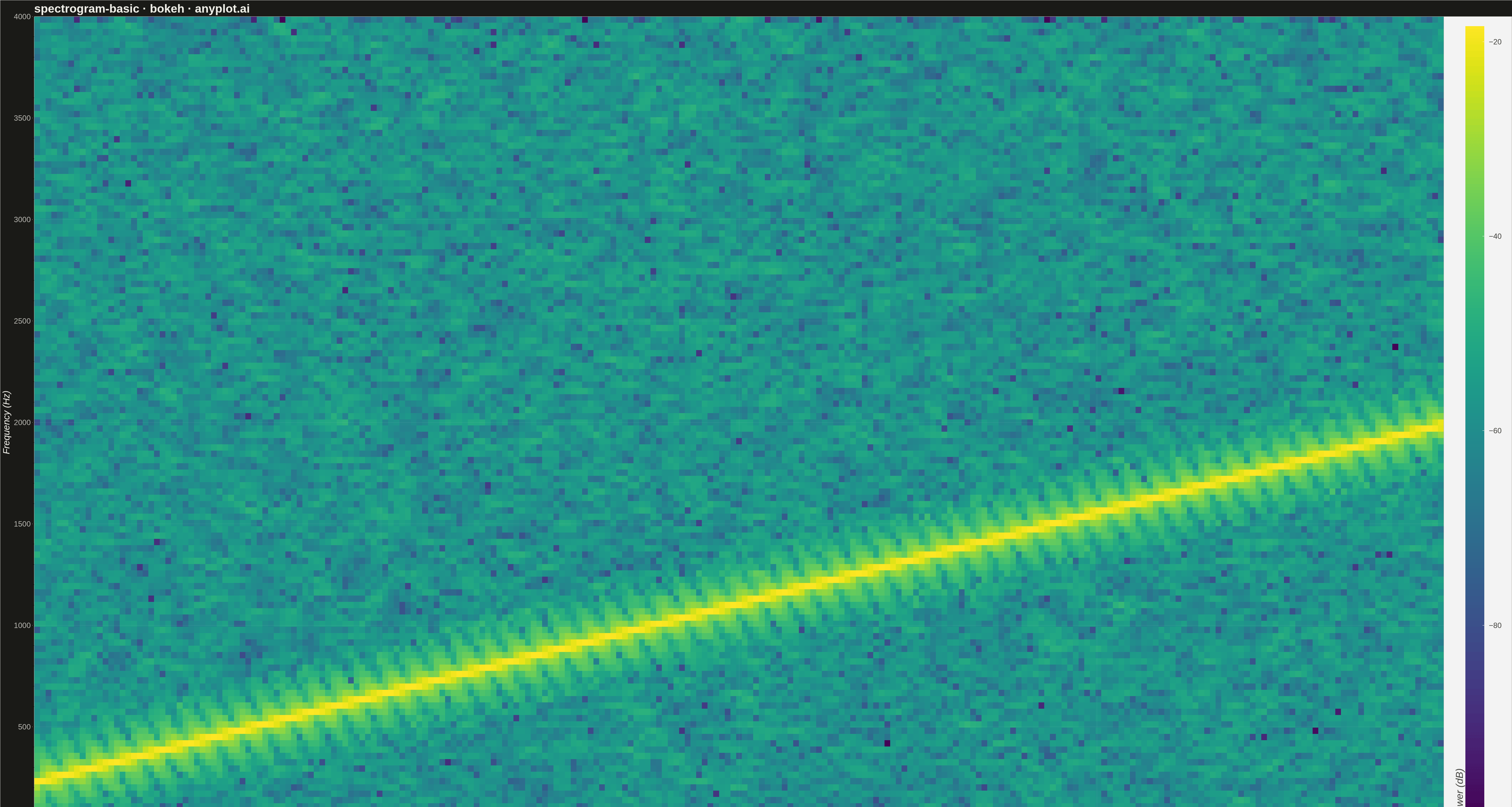
A spectrogram displaying time-frequency representation of a signal as a heatmap. It shows how the frequency content of a signal changes over time, with color intensity representing the amplitude or power at each time-frequency point. Essential for analyzing non-stationary signals where frequency characteristics vary, revealing patterns invisible in time-domain or frequency-domain views alone.
""" anyplot.ai
spectrogram-basic: Spectrogram Time-Frequency Heatmap
Library: bokeh 3.9.0 | Python 3.13.13
Quality: 90/100 | Updated: 2026-05-15
"""

import os
import time
from pathlib import Path

import numpy as np
from bokeh.io import output_file, save
from bokeh.models import BasicTicker, ColorBar, LinearColorMapper
from bokeh.palettes import Viridis256
from bokeh.plotting import figure
from scipy import signal
from selenium import webdriver
from selenium.webdriver.chrome.options import Options


THEME = os.getenv("ANYPLOT_THEME", "light")
PAGE_BG = "#FAF8F1" if THEME == "light" else "#1A1A17"
ELEVATED_BG = "#FFFDF6" if THEME == "light" else "#242420"
INK = "#1A1A17" if THEME == "light" else "#F0EFE8"
INK_SOFT = "#4A4A44" if THEME == "light" else "#B8B7B0"

# Data - Generate chirp signal with increasing frequency
np.random.seed(42)
sample_rate = 8000
duration = 2.0
t = np.linspace(0, duration, int(sample_rate * duration), endpoint=False)

f0 = 200
f1 = 2000
chirp_signal = signal.chirp(t, f0, duration, f1, method="linear")
chirp_signal += 0.1 * np.random.randn(len(chirp_signal))

# Compute spectrogram
nperseg = 256
noverlap = 192
frequencies, times, Sxx = signal.spectrogram(
    chirp_signal, fs=sample_rate, nperseg=nperseg, noverlap=noverlap, scaling="density"
)

Sxx_db = 10 * np.log10(Sxx + 1e-10)

# Create figure
p = figure(
    width=4800,
    height=2700,
    title="spectrogram-basic · bokeh · anyplot.ai",
    x_axis_label="Time (seconds)",
    y_axis_label="Frequency (Hz)",
    x_range=(times.min(), times.max()),
    y_range=(frequencies.min(), frequencies.max()),
    tools="",
    toolbar_location=None,
)

# Color mapping
color_mapper = LinearColorMapper(palette=Viridis256, low=Sxx_db.min(), high=Sxx_db.max())

# Render spectrogram
p.image(
    image=[Sxx_db],
    x=times.min(),
    y=frequencies.min(),
    dw=times.max() - times.min(),
    dh=frequencies.max() - frequencies.min(),
    color_mapper=color_mapper,
    level="image",
)

# Colorbar
color_bar = ColorBar(
    color_mapper=color_mapper,
    ticker=BasicTicker(),
    label_standoff=15,
    border_line_color=INK_SOFT,
    location=(0, 0),
    title="Power (dB)",
    title_text_font_size="24pt",
    major_label_text_font_size="18pt",
    width=60,
    padding=30,
)
p.add_layout(color_bar, "right")

# Text styling
p.title.text_font_size = "28pt"
p.title.text_color = INK
p.xaxis.axis_label_text_font_size = "22pt"
p.yaxis.axis_label_text_font_size = "22pt"
p.xaxis.axis_label_text_color = INK
p.yaxis.axis_label_text_color = INK
p.xaxis.major_label_text_font_size = "18pt"
p.yaxis.major_label_text_font_size = "18pt"
p.xaxis.major_label_text_color = INK_SOFT
p.yaxis.major_label_text_color = INK_SOFT

# Axes and grid
p.xaxis.axis_line_color = INK_SOFT
p.yaxis.axis_line_color = INK_SOFT
p.xaxis.major_tick_line_color = INK_SOFT
p.yaxis.major_tick_line_color = INK_SOFT
p.xgrid.grid_line_color = INK
p.ygrid.grid_line_color = INK
p.xgrid.grid_line_alpha = 0.10
p.ygrid.grid_line_alpha = 0.10

# Background
p.background_fill_color = PAGE_BG
p.border_fill_color = PAGE_BG
p.outline_line_color = INK_SOFT

# Legend styling
if p.legend:
    p.legend.background_fill_color = ELEVATED_BG
    p.legend.border_line_color = INK_SOFT
    p.legend.label_text_color = INK_SOFT

# Save HTML
output_file(f"plot-{THEME}.html")
save(p)

# Screenshot with Selenium
W, H = 4800, 2700
opts = Options()
for arg in (
    "--headless=new",
    "--no-sandbox",
    "--disable-dev-shm-usage",
    "--disable-gpu",
    f"--window-size={W},{H}",
    "--hide-scrollbars",
):
    opts.add_argument(arg)
driver = webdriver.Chrome(options=opts)
driver.set_window_size(W, H)
driver.get(f"file://{Path(f'plot-{THEME}.html').resolve()}")
time.sleep(3)
driver.save_screenshot(f"plot-{THEME}.png")
driver.quit()
Runnable source as JSON, for any HTTP client: https://api.anyplot.ai/specs/spectrogram-basic/bokeh/code. Any spec id and library id listed in llms-full.txt fit the same URL shape; every URL below is complete and callable.
{
  "spec_id": "spectrogram-basic",
  "language": "python",
  "library": "bokeh",
  "page": "https://anyplot.ai/spectrogram-basic/python/bokeh",
  "hub": "https://anyplot.ai/spectrogram-basic",
  "code_json": "https://api.anyplot.ai/specs/spectrogram-basic/bokeh/code",
  "spec_json": "https://api.anyplot.ai/specs/spectrogram-basic",
  "render_light_png": "https://storage.googleapis.com/anyplot-images/plots/spectrogram-basic/python/bokeh/plot-light.png",
  "render_dark_png": "https://storage.googleapis.com/anyplot-images/plots/spectrogram-basic/python/bokeh/plot-dark.png",
  "interactive_light_html": "https://storage.googleapis.com/anyplot-images/plots/spectrogram-basic/python/bokeh/plot-light.html",
  "interactive_dark_html": "https://storage.googleapis.com/anyplot-images/plots/spectrogram-basic/python/bokeh/plot-dark.html",
  "quality_score": 90.0,
  "license": "MIT",
  "guide": "https://anyplot.ai/llms.txt"
}
Part of Spectrogram Time-Frequency Heatmap on anyplot.ai.