The same plot in 14 other libraries — Python: Altair, Bokeh, lets-plot, Matplotlib, Plotly, plotnine, Pygal, Seaborn; Julia: Makie.jl; JavaScript: Chart.js, D3.js, Apache ECharts, Highcharts, MUI X Charts. Compare all 15 side by side: Spectrogram Time-Frequency Heatmap in Python, R, Julia and JavaScript.
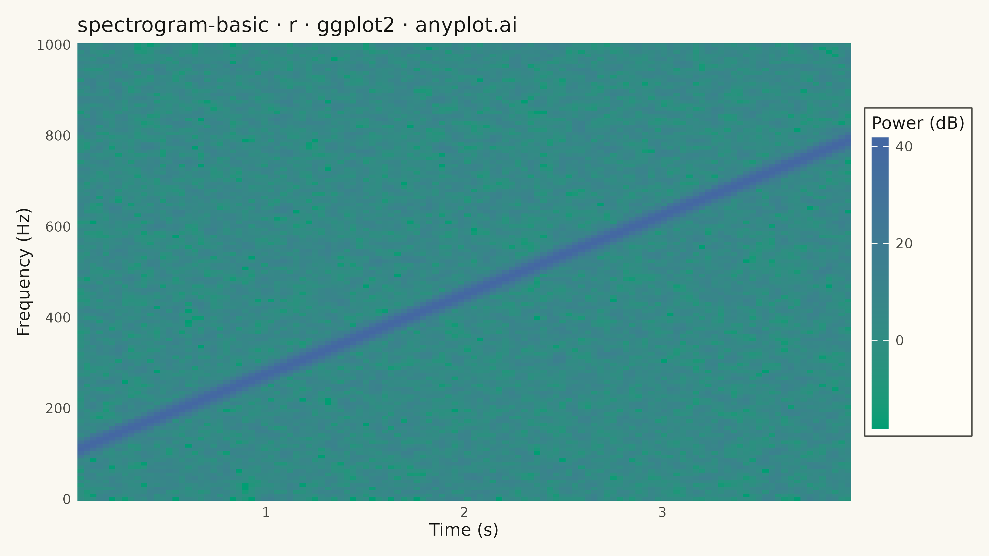
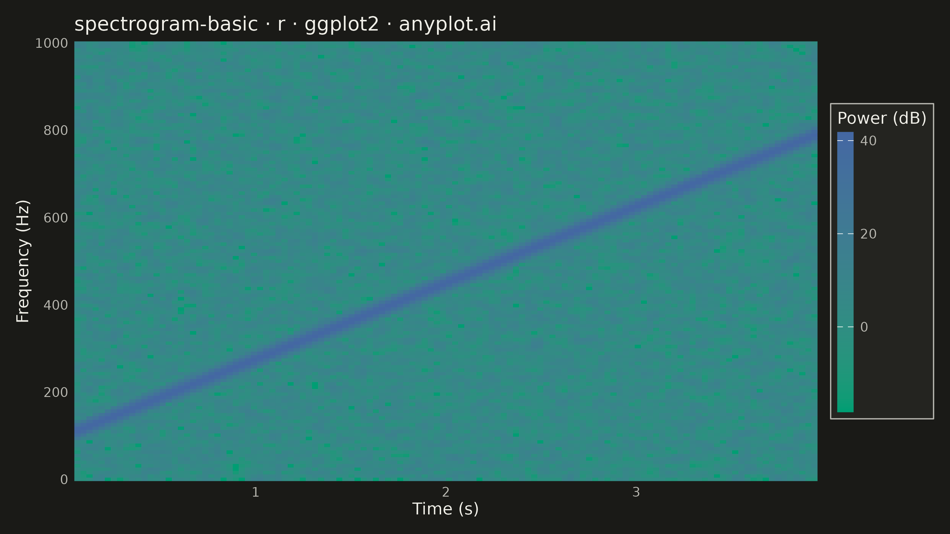
A spectrogram displaying time-frequency representation of a signal as a heatmap. It shows how the frequency content of a signal changes over time, with color intensity representing the amplitude or power at each time-frequency point. Essential for analyzing non-stationary signals where frequency characteristics vary, revealing patterns invisible in time-domain or frequency-domain views alone.
#' anyplot.ai
#' spectrogram-basic: Spectrogram Time-Frequency Heatmap
#' Library: ggplot2 3.5.1 | R 4.4.1
#' Quality: 87/100 | Created: 2026-09-09

library(ggplot2)
library(ragg)

set.seed(42)

# --- Theme tokens -----------------------------------------------------------
THEME       <- Sys.getenv("ANYPLOT_THEME", "light")
PAGE_BG     <- if (THEME == "light") "#FAF8F1" else "#1A1A17"
ELEVATED_BG <- if (THEME == "light") "#FFFDF6" else "#242420"
INK         <- if (THEME == "light") "#1A1A17" else "#F0EFE8"
INK_SOFT    <- if (THEME == "light") "#4A4A44" else "#B8B7B0"

# --- Data: synthetic linear chirp signal ------------------------------------
sample_rate <- 4000
duration <- 4
n_samples <- sample_rate * duration
t <- seq_len(n_samples) / sample_rate

freq_start <- 100
freq_end <- 800
instantaneous_phase <- 2 * pi * (freq_start * t + (freq_end - freq_start) * t^2 / (2 * duration))
signal <- sin(instantaneous_phase) + 0.15 * rnorm(n_samples)

# --- Short-time Fourier transform (Hann window, 75% overlap) ---------------
window_size <- 512
hop <- 128
hann_window <- 0.5 - 0.5 * cos(2 * pi * (0:(window_size - 1)) / (window_size - 1))

n_windows <- floor((n_samples - window_size) / hop) + 1
n_freq_bins <- window_size %/% 2 + 1

freqs <- (0:(n_freq_bins - 1)) * sample_rate / window_size
times <- ((0:(n_windows - 1)) * hop + window_size / 2) / sample_rate

power_db <- matrix(0, nrow = n_windows, ncol = n_freq_bins)
for (i in seq_len(n_windows)) {
  start <- (i - 1) * hop + 1
  segment <- signal[start:(start + window_size - 1)] * hann_window
  spectrum <- fft(segment)[1:n_freq_bins]
  power_db[i, ] <- 20 * log10(Mod(spectrum) + 1e-6)
}

# Light separable 3-tap smoothing (time then frequency) quiets salt-and-pepper
# noise-floor speckle without blurring the ridge, which spans many bins.
smooth_1d <- function(v) {
  n <- length(v)
  c(v[1], (v[1:(n - 2)] + v[2:(n - 1)] + v[3:n]) / 3, v[n])
}
power_db <- t(apply(power_db, 1, smooth_1d))
power_db <- apply(power_db, 2, smooth_1d)

dynamic_range_db <- 48
power_db <- pmax(power_db, max(power_db) - dynamic_range_db)

max_freq_display <- 1000
freq_display_idx <- which(freqs <= max_freq_display)

spec_df <- data.frame(
  time = rep(times, times = length(freq_display_idx)),
  frequency = rep(freqs[freq_display_idx], each = n_windows),
  power = as.vector(power_db[, freq_display_idx])
)

# Ridge trace: the peak-power frequency at each time step, from the real STFT
# data (not a fitted curve) — a second ggplot2 layer beyond the raster.
ridge_df <- data.frame(
  time = times,
  frequency = freqs[freq_display_idx][apply(power_db[, freq_display_idx, drop = FALSE], 1, which.max)]
)

overlap_pct <- round((window_size - hop) / window_size * 100)

# --- Plot ---------------------------------------------------------------
title_str <- "spectrogram-basic · r · ggplot2 · anyplot.ai"
title_fontsize <- round(12 * min(1.0, 67 / nchar(title_str)))
subtitle_str <- sprintf(
  "Hann window, %d samples · %d-sample hop (%d%% overlap) · %d dB dynamic range",
  window_size, hop, overlap_pct, dynamic_range_db
)

p <- ggplot(spec_df, aes(x = time, y = frequency, fill = power)) +
  geom_raster() +
  geom_line(
    data = ridge_df, aes(x = time, y = frequency),
    inherit.aes = FALSE, color = INK, linewidth = 0.35, alpha = 0.55
  ) +
  scale_fill_gradient(
    low = "#009E73", high = "#4467A3",
    name = "Power (dB)",
    guide = guide_colorbar(barwidth = unit(0.35, "cm"), barheight = unit(6, "cm"))
  ) +
  scale_x_continuous(expand = c(0, 0), breaks = seq(0, duration, 1)) +
  scale_y_continuous(expand = c(0, 0), breaks = seq(0, max_freq_display, 200)) +
  labs(x = "Time (s)", y = "Frequency (Hz)", title = title_str, subtitle = subtitle_str) +
  theme_minimal(base_size = 8) +
  theme(
    plot.background   = element_rect(fill = PAGE_BG, color = PAGE_BG),
    panel.background  = element_rect(fill = PAGE_BG, color = NA),
    panel.grid        = element_blank(),
    axis.ticks        = element_blank(),
    axis.title        = element_text(color = INK, size = 10),
    axis.text         = element_text(color = INK_SOFT, size = 8),
    plot.title        = element_text(color = INK, size = title_fontsize),
    plot.subtitle     = element_text(color = INK_SOFT, size = 8),
    legend.background = element_rect(fill = ELEVATED_BG, color = INK_SOFT),
    legend.text       = element_text(color = INK_SOFT, size = 8),
    legend.title      = element_text(color = INK, size = 10),
    plot.margin       = margin(10, 10, 10, 10)
  )

# --- Save -------------------------------------------------------------------
ggsave(
  filename = sprintf("plot-%s.png", THEME),
  plot     = p,
  device   = ragg::agg_png,
  width    = 8,
  height   = 4.5,
  units    = "in",
  dpi      = 400
)
Runnable source as JSON, for any HTTP client: https://api.anyplot.ai/specs/spectrogram-basic/ggplot2/code. Any spec id and library id listed in llms-full.txt fit the same URL shape; every URL below is complete and callable.
{
  "spec_id": "spectrogram-basic",
  "language": "r",
  "library": "ggplot2",
  "page": "https://anyplot.ai/spectrogram-basic/r/ggplot2",
  "hub": "https://anyplot.ai/spectrogram-basic",
  "code_json": "https://api.anyplot.ai/specs/spectrogram-basic/ggplot2/code",
  "spec_json": "https://api.anyplot.ai/specs/spectrogram-basic",
  "render_light_png": "https://storage.googleapis.com/anyplot-images/plots/spectrogram-basic/r/ggplot2/plot-light.png",
  "render_dark_png": "https://storage.googleapis.com/anyplot-images/plots/spectrogram-basic/r/ggplot2/plot-dark.png",
  "quality_score": 87.0,
  "license": "MIT",
  "guide": "https://anyplot.ai/llms.txt"
}
Part of Spectrogram Time-Frequency Heatmap on anyplot.ai.