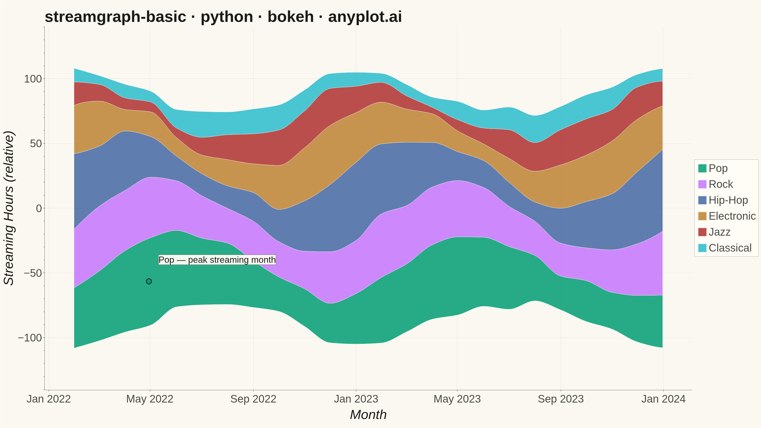
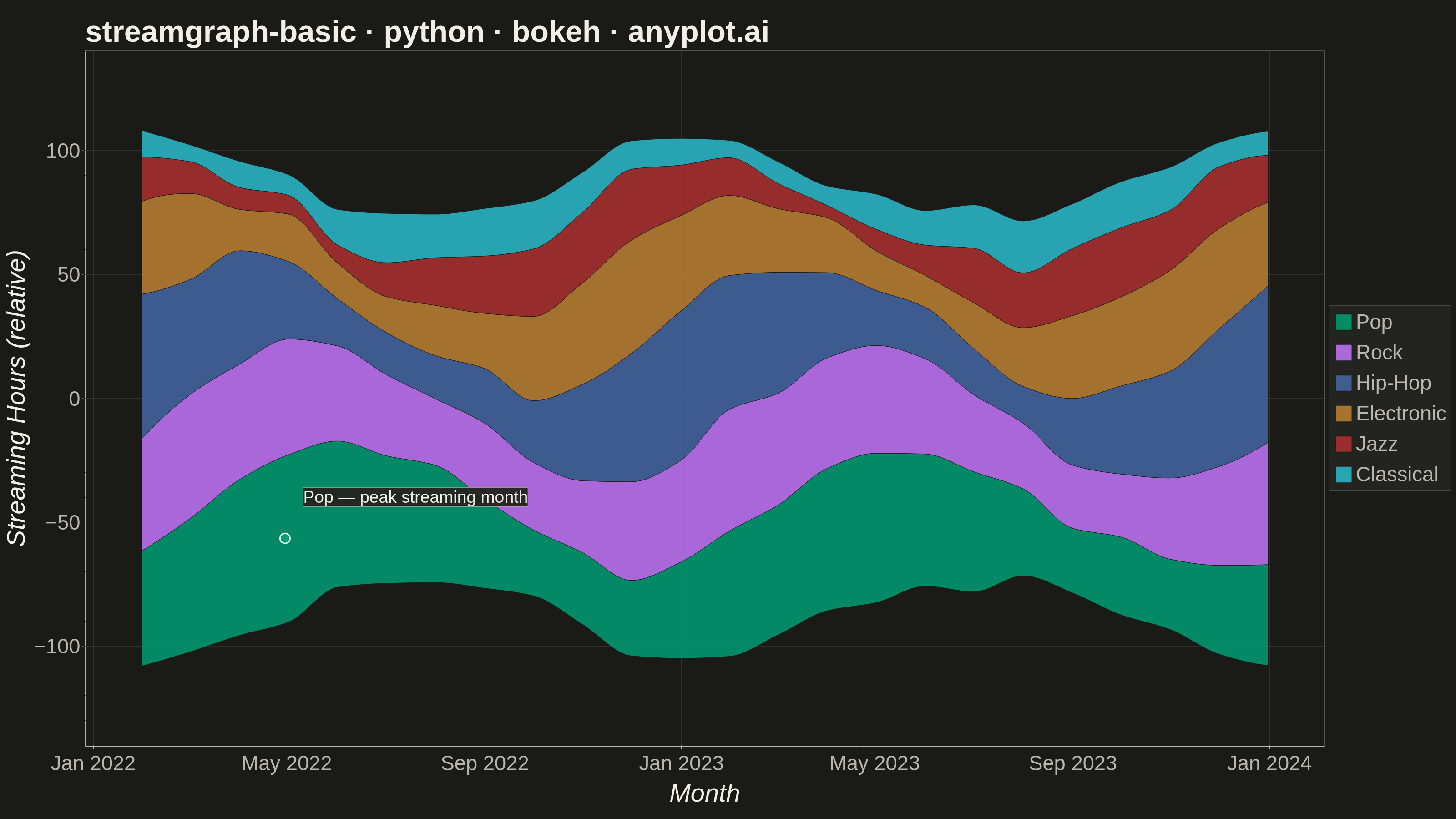
A streamgraph (also known as a stacked area chart with a centered baseline) displaying the composition of multiple categories over time with smooth, flowing curves. Unlike traditional stacked area charts, streamgraphs use a symmetric baseline centered around the x-axis, creating an organic, river-like appearance that emphasizes the overall shape and relative proportions of each category while minimizing the visual distortion of individual layers.
""" anyplot.ai
streamgraph-basic: Basic Stream Graph
Library: bokeh 3.9.2 | Python 3.13.14
Quality: 89/100 | Updated: 2026-08-05
"""

import os
import time
from pathlib import Path

import numpy as np
import pandas as pd
from bokeh.io import output_file, save
from bokeh.models import ColumnDataSource, HoverTool, Label, Legend, Range1d
from bokeh.plotting import figure
from scipy.interpolate import PchipInterpolator
from selenium import webdriver
from selenium.webdriver.chrome.options import Options


# Theme tokens
THEME = os.getenv("ANYPLOT_THEME", "light")
PAGE_BG = "#FAF8F1" if THEME == "light" else "#1A1A17"
ELEVATED_BG = "#FFFDF6" if THEME == "light" else "#242420"
INK = "#1A1A17" if THEME == "light" else "#F0EFE8"
INK_SOFT = "#4A4A44" if THEME == "light" else "#B8B7B0"

# Imprint palette — first series always #009E73
COLORS = ["#009E73", "#C475FD", "#4467A3", "#BD8233", "#AE3030", "#2ABCCD"]

# Data: monthly streaming hours by music genre over two years
np.random.seed(42)

months = pd.date_range(start="2022-01-01", periods=24, freq="ME")
categories = ["Pop", "Rock", "Hip-Hop", "Electronic", "Jazz", "Classical"]

n_points = len(months)
base = np.linspace(0, 4 * np.pi, n_points)

raw = {
    "Pop": 45 + 18 * np.sin(base) + np.random.randn(n_points) * 3,
    "Rock": 38 + 12 * np.sin(base + 0.8) + np.random.randn(n_points) * 2.5,
    "Hip-Hop": 35 + 22 * np.sin(base + 1.6) + np.random.randn(n_points) * 4,
    "Electronic": 28 + 14 * np.sin(base + 2.4) + np.random.randn(n_points) * 2.5,
    "Jazz": 18 + 10 * np.sin(base + 3.2) + np.random.randn(n_points) * 2,
    "Classical": 14 + 6 * np.sin(base + 4.0) + np.random.randn(n_points) * 1.5,
}

for cat in categories:
    raw[cat] = np.maximum(raw[cat], 5)

df = pd.DataFrame(raw)

# Symmetric baseline — center the stack around zero
values = df[categories].values
total = values.sum(axis=1)
baseline_offset = total / 2

y_bottom = np.zeros_like(values)
y_top = np.zeros_like(values)
for i in range(len(categories)):
    if i == 0:
        y_bottom[:, i] = -baseline_offset
        y_top[:, i] = y_bottom[:, i] + values[:, i]
    else:
        y_bottom[:, i] = y_top[:, i - 1]
        y_top[:, i] = y_bottom[:, i] + values[:, i]

# Smooth interpolation for flowing curves.
# PCHIP (monotone cubic Hermite) is shape-preserving and does not overshoot at
# the series edges the way a high-degree polynomial fit (Runge phenomenon) does.
x_numeric = np.arange(n_points)
n_smooth = n_points * 10
x_smooth = np.linspace(0, n_points - 1, n_smooth)

months_smooth = pd.date_range(start=months.min(), end=months.max(), periods=n_smooth)
y_bottom_smooth = np.zeros((n_smooth, len(categories)))
y_top_smooth = np.zeros((n_smooth, len(categories)))

for i in range(len(categories)):
    y_bottom_smooth[:, i] = PchipInterpolator(x_numeric, y_bottom[:, i])(x_smooth)
    y_top_smooth[:, i] = PchipInterpolator(x_numeric, y_top[:, i])(x_smooth)

# Extra headroom above/below the widest point of the stack so the bands don't
# crowd the top/bottom plot edges.
max_disp = np.max(baseline_offset)
y_limit = max_disp * 1.3

# Plot
p = figure(
    width=3200,
    height=1800,
    title="streamgraph-basic · python · bokeh · anyplot.ai",
    x_axis_label="Month",
    y_axis_label="Streaming Hours (relative)",
    x_axis_type="datetime",
    toolbar_location=None,
    min_border_bottom=160,
    min_border_left=180,
    min_border_top=110,
    min_border_right=50,
)
p.y_range = Range1d(start=-y_limit, end=y_limit)

# Font sizes for 3200×1800 px canvas
p.title.text_font_size = "50pt"
p.title.text_color = INK
p.xaxis.axis_label_text_font_size = "42pt"
p.yaxis.axis_label_text_font_size = "42pt"
p.xaxis.major_label_text_font_size = "34pt"
p.yaxis.major_label_text_font_size = "34pt"

# Theme-adaptive chrome
p.background_fill_color = PAGE_BG
p.border_fill_color = PAGE_BG
p.outline_line_color = None
p.xaxis.axis_label_text_color = INK
p.yaxis.axis_label_text_color = INK
p.xaxis.major_label_text_color = INK_SOFT
p.yaxis.major_label_text_color = INK_SOFT
p.xaxis.axis_line_color = INK_SOFT
p.yaxis.axis_line_color = INK_SOFT
p.xaxis.major_tick_line_color = INK_SOFT
p.yaxis.major_tick_line_color = INK_SOFT
p.xgrid.grid_line_color = INK
p.ygrid.grid_line_color = INK
p.xgrid.grid_line_alpha = 0.10
p.ygrid.grid_line_alpha = 0.10

# Draw streamgraph patches
x_values = months_smooth.values
legend_items = []
hover_renderers = []

for i, cat in enumerate(categories):
    xs = np.concatenate([x_values, x_values[::-1]])
    ys = np.concatenate([y_top_smooth[:, i], y_bottom_smooth[:, i][::-1]])

    source = ColumnDataSource(data={"x": xs, "y": ys, "genre": [cat] * len(xs)})
    renderer = p.patch(
        x="x", y="y", source=source, fill_color=COLORS[i], fill_alpha=0.85, line_color=PAGE_BG, line_width=1
    )
    legend_items.append((cat, [renderer]))
    hover_renderers.append(renderer)

# HoverTool — shows genre name on hover
hover = HoverTool(renderers=hover_renderers, tooltips=[("Genre", "@genre")])
p.add_tools(hover)

# Legend outside the plot area
legend = Legend(items=legend_items, location="center")
legend.label_text_font_size = "34pt"
legend.label_text_color = INK_SOFT
legend.glyph_height = 44
legend.glyph_width = 44
legend.spacing = 15
legend.background_fill_color = ELEVATED_BG
legend.border_line_color = INK_SOFT
p.add_layout(legend, "right")

# Focal-point callout on the genre with the highest peak streaming month —
# gives the chart a storytelling anchor instead of leaving all six bands
# equally weighted.
peak_genre = "Pop"
peak_idx = int(np.argmax(raw[peak_genre]))
peak_x = months[peak_idx]
peak_y = (y_top[peak_idx, 0] + y_bottom[peak_idx, 0]) / 2

peak_marker_source = ColumnDataSource(data={"x": [peak_x], "y": [peak_y]})
p.scatter(x="x", y="y", source=peak_marker_source, size=22, fill_color=COLORS[0], line_color=INK, line_width=3)

peak_label = Label(
    x=peak_x,
    y=peak_y,
    x_offset=40,
    y_offset=70,
    text=f"{peak_genre} — peak streaming month",
    text_font_size="28pt",
    text_color=INK,
    background_fill_color=ELEVATED_BG,
    background_fill_alpha=0.95,
    border_line_color=INK_SOFT,
    border_line_width=1,
)
p.add_layout(peak_label)

# Save interactive HTML
output_file(f"plot-{THEME}.html")
save(p)

# Screenshot with headless Chrome (export_png unavailable in this environment)
W, H = 3200, 1800
opts = Options()
for arg in (
    "--headless=new",
    "--no-sandbox",
    "--disable-dev-shm-usage",
    "--disable-gpu",
    f"--window-size={W},{H}",
    "--hide-scrollbars",
):
    opts.add_argument(arg)

driver = webdriver.Chrome(options=opts)
driver.set_window_size(W, H)
driver.get(f"file://{Path(f'plot-{THEME}.html').resolve()}")
driver.execute_cdp_cmd(
    "Emulation.setDeviceMetricsOverride", {"width": W, "height": H, "deviceScaleFactor": 1, "mobile": False}
)
time.sleep(3)
driver.save_screenshot(f"plot-{THEME}.png")
driver.quit()
Runnable source as JSON, for any HTTP client: https://api.anyplot.ai/specs/streamgraph-basic/bokeh/code. Any spec id and library id listed in llms-full.txt fit the same URL shape; every URL below is complete and callable.
{
  "spec_id": "streamgraph-basic",
  "language": "python",
  "library": "bokeh",
  "page": "https://anyplot.ai/streamgraph-basic/python/bokeh",
  "hub": "https://anyplot.ai/streamgraph-basic",
  "code_json": "https://api.anyplot.ai/specs/streamgraph-basic/bokeh/code",
  "spec_json": "https://api.anyplot.ai/specs/streamgraph-basic",
  "render_light_png": "https://storage.googleapis.com/anyplot-images/plots/streamgraph-basic/python/bokeh/plot-light.png",
  "render_dark_png": "https://storage.googleapis.com/anyplot-images/plots/streamgraph-basic/python/bokeh/plot-dark.png",
  "interactive_light_html": "https://storage.googleapis.com/anyplot-images/plots/streamgraph-basic/python/bokeh/plot-light.html",
  "interactive_dark_html": "https://storage.googleapis.com/anyplot-images/plots/streamgraph-basic/python/bokeh/plot-dark.html",
  "quality_score": 89.0,
  "license": "MIT",
  "guide": "https://anyplot.ai/llms.txt"
}
Part of Basic Stream Graph on anyplot.ai.