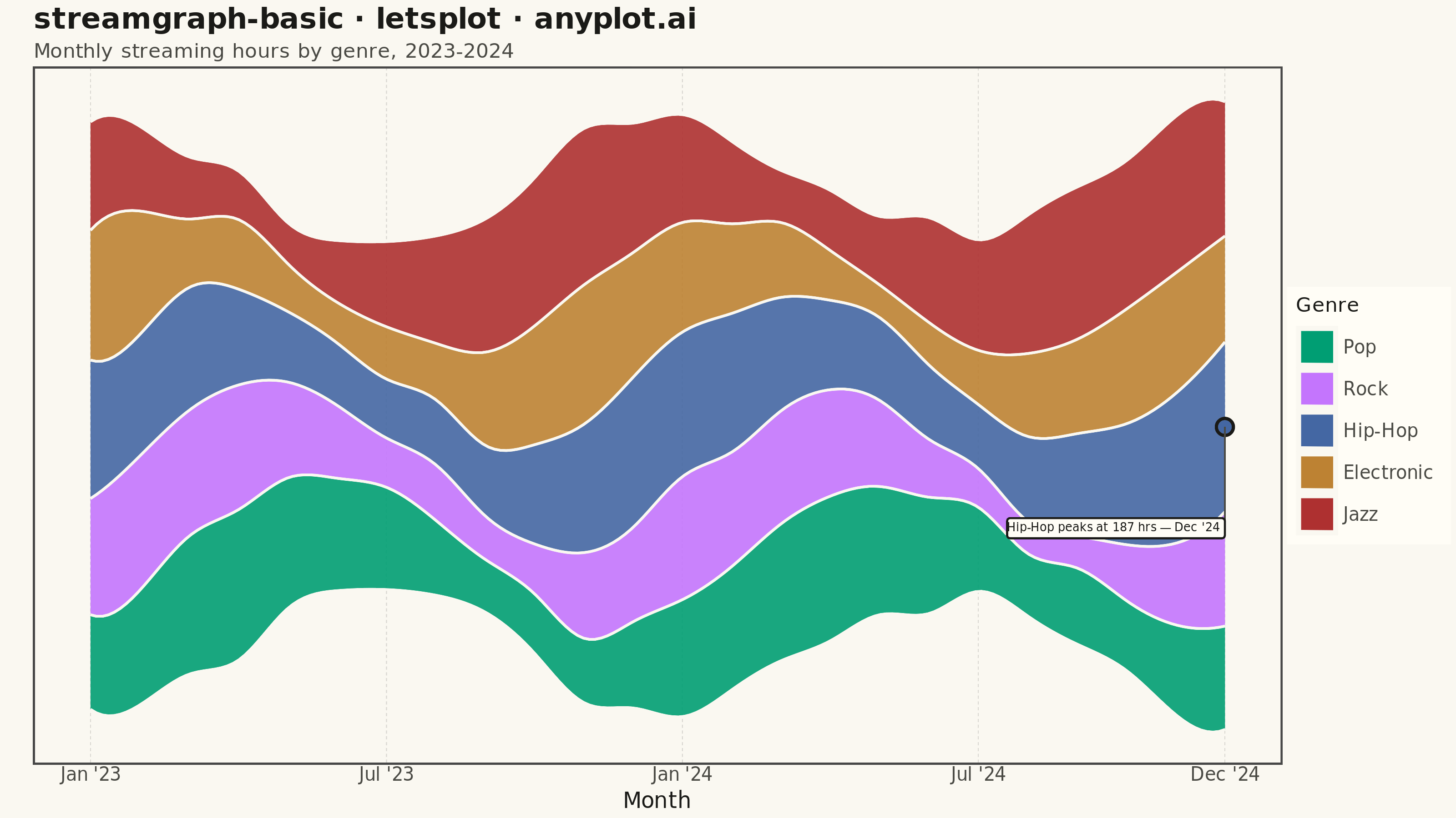
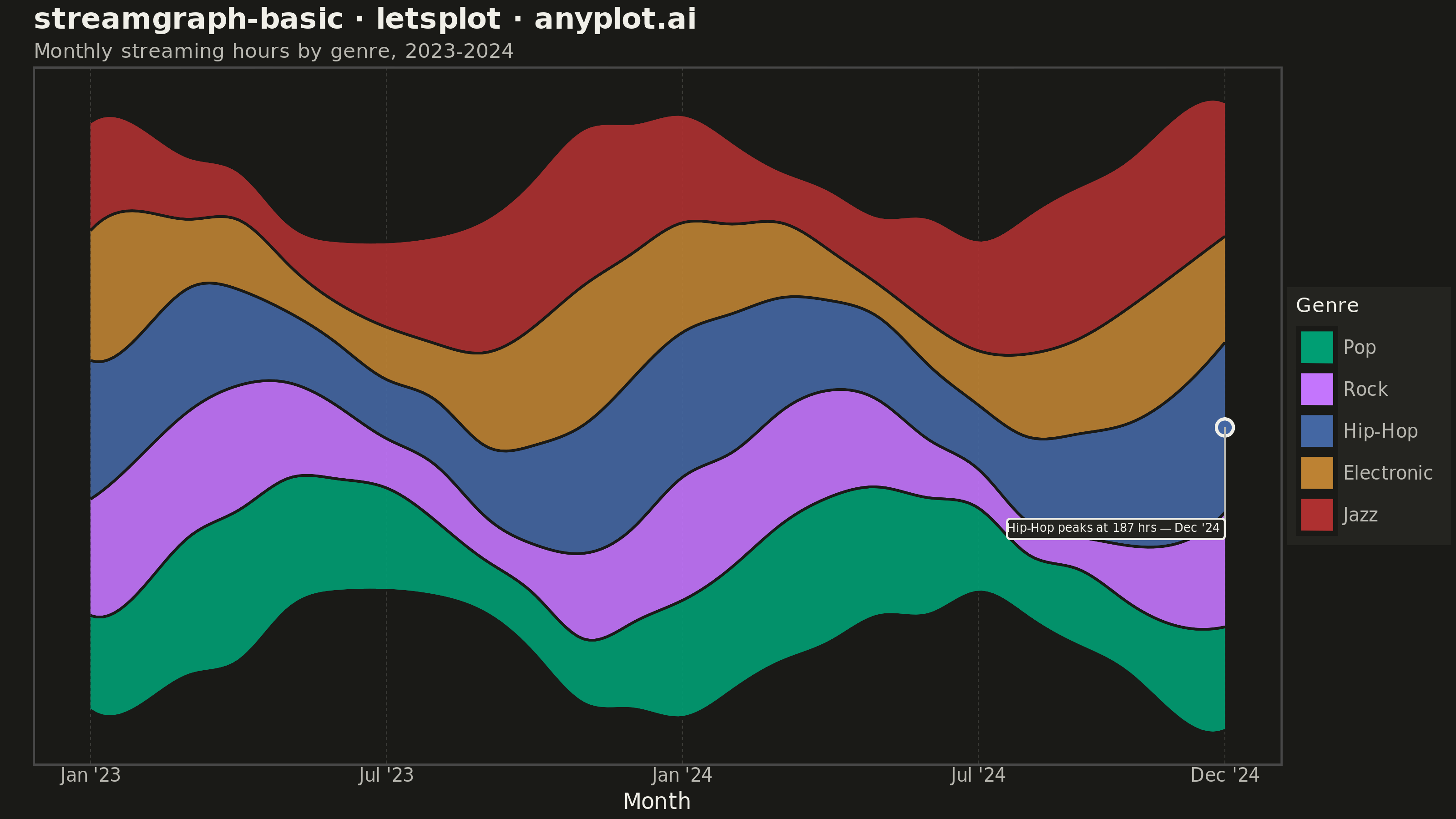
A streamgraph (also known as a stacked area chart with a centered baseline) displaying the composition of multiple categories over time with smooth, flowing curves. Unlike traditional stacked area charts, streamgraphs use a symmetric baseline centered around the x-axis, creating an organic, river-like appearance that emphasizes the overall shape and relative proportions of each category while minimizing the visual distortion of individual layers.
""" anyplot.ai
streamgraph-basic: Basic Stream Graph
Library: letsplot 4.11.0 | Python 3.13.14
Quality: 91/100 | Updated: 2026-08-05
"""

import os

import numpy as np
import pandas as pd
from lets_plot import *
from lets_plot.export import ggsave
from scipy.interpolate import make_interp_spline


LetsPlot.setup_html()

# Theme tokens
THEME = os.getenv("ANYPLOT_THEME", "light")
PAGE_BG = "#FAF8F1" if THEME == "light" else "#1A1A17"
ELEVATED_BG = "#FFFDF6" if THEME == "light" else "#242420"
INK = "#1A1A17" if THEME == "light" else "#F0EFE8"
INK_SOFT = "#4A4A44" if THEME == "light" else "#B8B7B0"
RULE = "rgba(26,26,23,0.15)" if THEME == "light" else "rgba(240,239,232,0.15)"

# Imprint palette — first series always #009E73
IMPRINT = ["#009E73", "#C475FD", "#4467A3", "#BD8233", "#AE3030"]

# Data — monthly streaming hours by music genre over two years
np.random.seed(42)
n_months = 24
genres = ["Pop", "Rock", "Hip-Hop", "Electronic", "Jazz"]
month_labels = pd.date_range("2023-01-01", periods=n_months, freq="MS").strftime("%b '%y")

raw_values = {}
months_orig = np.arange(n_months, dtype=float)
for i, genre in enumerate(genres):
    base = 100 + 50 * np.sin(np.linspace(0, 4 * np.pi, n_months) + i * 0.7)
    trend = np.linspace(0, 25, n_months) * (1 if i % 2 == 0 else -0.6)
    noise = np.random.randn(n_months) * 8
    raw_values[genre] = np.clip(base + trend + noise, 25, None)

# Smooth each series with a cubic spline for flowing curves
n_interp = n_months * 8
months_smooth = np.linspace(0, n_months - 1, n_interp)
values_smooth = {}
for genre in genres:
    spline = make_interp_spline(months_orig, raw_values[genre], k=3)
    values_smooth[genre] = np.clip(spline(months_smooth), 10, None)

# Compute streamgraph positions (symmetric baseline around zero)
values_matrix = np.array([values_smooth[g] for g in genres])
total_per_point = values_matrix.sum(axis=0)
baseline_offset = -total_per_point / 2

data = []
for t_idx, t in enumerate(months_smooth):
    cumulative = baseline_offset[t_idx]
    month_lbl = month_labels[int(round(t))]
    for genre_idx, genre in enumerate(genres):
        value = values_matrix[genre_idx, t_idx]
        ymin = cumulative
        ymax = cumulative + value
        data.append({"month": t, "genre": genre, "ymin": ymin, "ymax": ymax, "value": value, "month_label": month_lbl})
        cumulative = ymax

df = pd.DataFrame(data)

# Focal point: the single month/genre combination with the highest streaming
# volume, called out with a label — gives the reader a concrete entry point
# into the data instead of five equally-weighted ribbons (DE-03)
peak = df.loc[df["value"].idxmax()]
peak_y = (peak["ymin"] + peak["ymax"]) / 2
range_all = df["ymax"].max() - df["ymin"].min()
label_direction = 1 if peak_y >= 0 else -1
peak_df = pd.DataFrame(
    {
        "month": [peak["month"]],
        "y": [peak_y],
        "label_y": [peak_y + label_direction * range_all * 0.16],
        "label": [f"{peak['genre']} peaks at {peak['value']:.0f} hrs — {peak['month_label']}"],
        "fill": [IMPRINT[genres.index(peak["genre"])]],
    }
)

# Plot
anyplot_theme = theme(
    plot_background=element_rect(fill=PAGE_BG, color=PAGE_BG),
    panel_background=element_rect(fill=PAGE_BG),
    panel_grid_major_x=element_line(color=RULE, size=0.4, linetype="dashed"),
    panel_grid_major_y=element_blank(),
    panel_grid_minor=element_blank(),
    axis_title=element_text(color=INK, size=12),
    axis_text=element_text(color=INK_SOFT, size=10),
    axis_text_y=element_blank(),
    axis_ticks_y=element_blank(),
    axis_line=element_line(color=INK_SOFT),
    plot_title=element_text(color=INK, size=16, face="bold"),
    plot_subtitle=element_text(color=INK_SOFT, size=11),
    legend_background=element_rect(fill=ELEVATED_BG, color=INK_SOFT),
    legend_text=element_text(color=INK_SOFT, size=10),
    legend_title=element_text(color=INK, size=11),
)

# lets-plot-distinctive touch: custom interactive tooltips on hover (HTML
# export) surfacing genre / month / hours per ribbon slice — not something a
# static grammar-of-graphics library (e.g. plotnine) can offer (LM-02)
tooltips = (
    layer_tooltips()
    .format("@value", ".0f")
    .line("Genre|@genre")
    .line("Month|@month_label")
    .line("Hours|@value")
)

plot = (
    ggplot(df, aes(x="month", fill="genre"))
    + geom_ribbon(
        aes(ymin="ymin", ymax="ymax"),
        alpha=0.9,
        color=PAGE_BG,
        size=0.6,
        tooltips=tooltips,
    )
    + geom_point(
        aes(x="month", y="y"),
        data=peak_df,
        color=INK,
        fill=peak_df["fill"].iloc[0],
        shape=21,
        size=3.5,
        inherit_aes=False,
    )
    + geom_segment(
        aes(x="month", y="y", xend="month", yend="label_y"),
        data=peak_df,
        color=INK_SOFT,
        size=0.4,
        inherit_aes=False,
    )
    + geom_label(
        aes(x="month", y="label_y", label="label"),
        data=peak_df,
        color=INK,
        fill=ELEVATED_BG,
        size=3.2,
        label_padding=0.4,
        hjust="inward",
        inherit_aes=False,
    )
    + scale_fill_manual(values=IMPRINT)
    + scale_x_continuous(
        breaks=[0, 6, 12, 18, 23], labels=["Jan '23", "Jul '23", "Jan '24", "Jul '24", "Dec '24"]
    )
    + labs(
        x="Month",
        y="",
        fill="Genre",
        title="streamgraph-basic · letsplot · anyplot.ai",
        subtitle="Monthly streaming hours by genre, 2023-2024",
    )
    + ggsize(800, 450)
    + theme_minimal()
    + anyplot_theme
)

# Save
ggsave(plot, filename=f"plot-{THEME}.png", path=".", scale=4)
ggsave(plot, filename=f"plot-{THEME}.html", path=".")
Runnable source as JSON, for any HTTP client: https://api.anyplot.ai/specs/streamgraph-basic/letsplot/code. Any spec id and library id listed in llms-full.txt fit the same URL shape; every URL below is complete and callable.
{
  "spec_id": "streamgraph-basic",
  "language": "python",
  "library": "letsplot",
  "page": "https://anyplot.ai/streamgraph-basic/python/letsplot",
  "hub": "https://anyplot.ai/streamgraph-basic",
  "code_json": "https://api.anyplot.ai/specs/streamgraph-basic/letsplot/code",
  "spec_json": "https://api.anyplot.ai/specs/streamgraph-basic",
  "render_light_png": "https://storage.googleapis.com/anyplot-images/plots/streamgraph-basic/python/letsplot/plot-light.png",
  "render_dark_png": "https://storage.googleapis.com/anyplot-images/plots/streamgraph-basic/python/letsplot/plot-dark.png",
  "interactive_light_html": "https://storage.googleapis.com/anyplot-images/plots/streamgraph-basic/python/letsplot/plot-light.html",
  "interactive_dark_html": "https://storage.googleapis.com/anyplot-images/plots/streamgraph-basic/python/letsplot/plot-dark.html",
  "quality_score": 91.0,
  "license": "MIT",
  "guide": "https://anyplot.ai/llms.txt"
}
Part of Basic Stream Graph on anyplot.ai.