The same plot in 14 other libraries — Python: Altair, Bokeh, lets-plot, Matplotlib, Plotly, plotnine, Pygal, Seaborn; Julia: Makie.jl; JavaScript: Chart.js, D3.js, Apache ECharts, Highcharts, MUI X Charts. Compare all 15 side by side: Basic Stream Graph in Python, R, Julia and JavaScript.
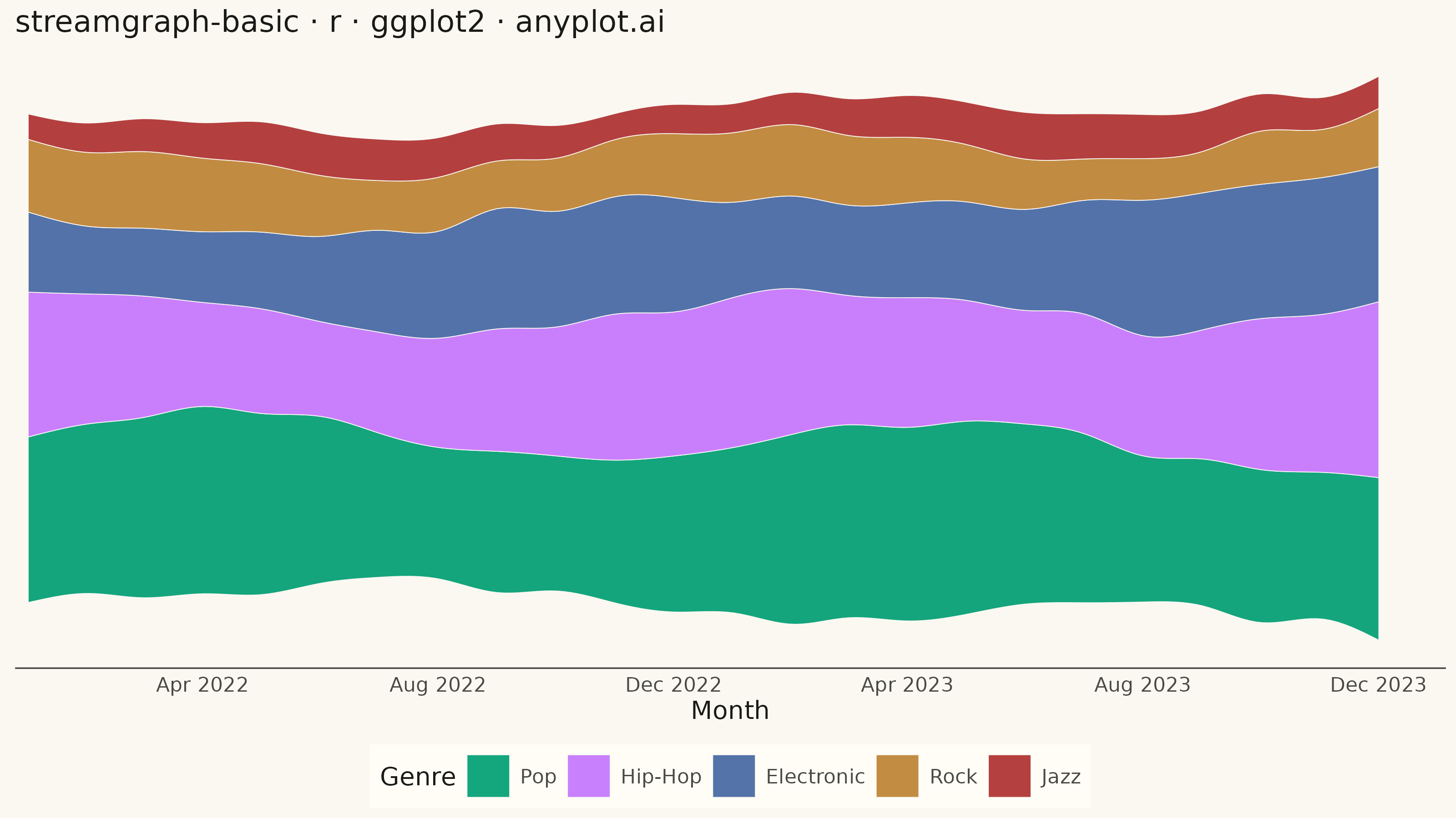
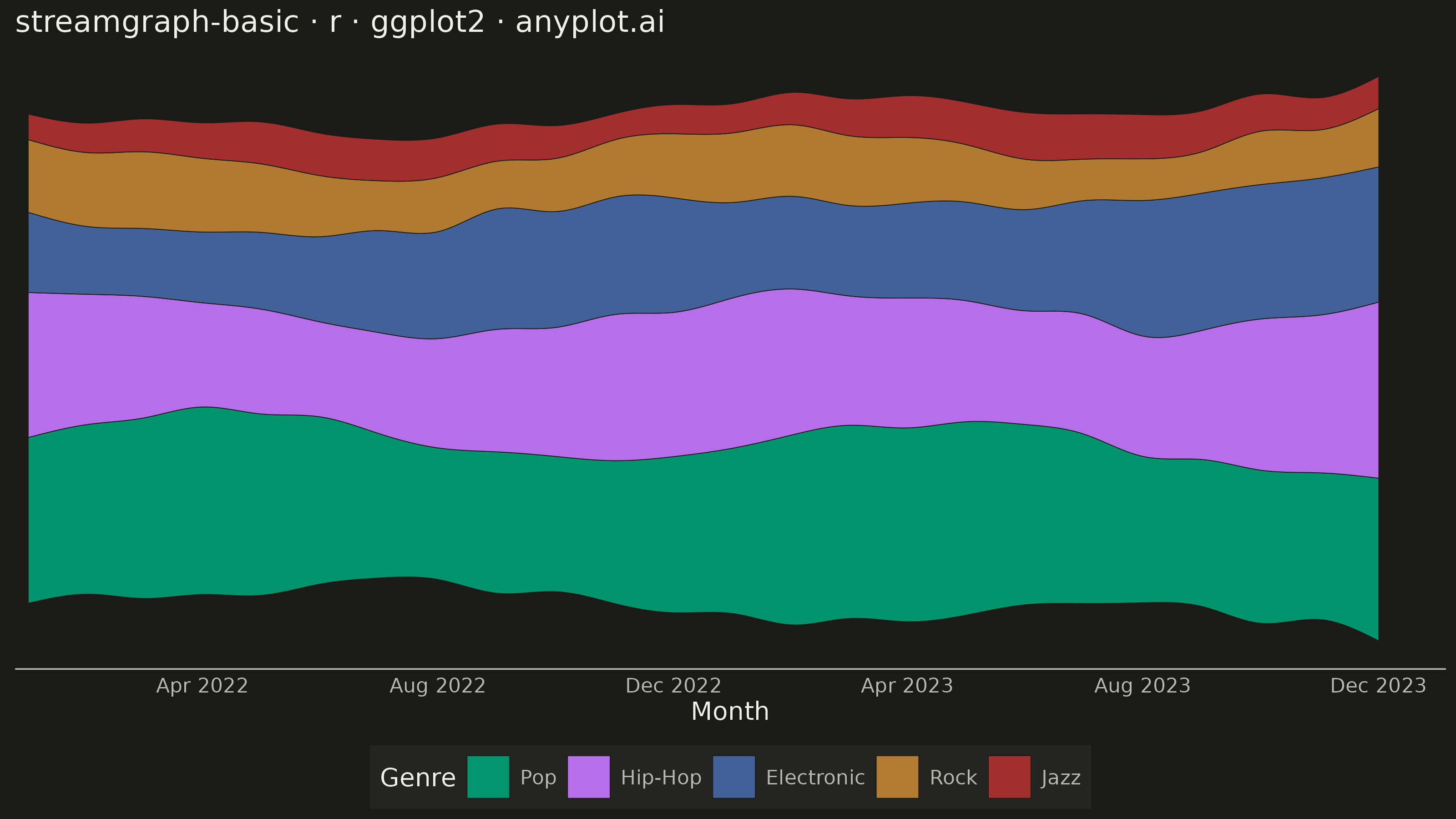
A streamgraph (also known as a stacked area chart with a centered baseline) displaying the composition of multiple categories over time with smooth, flowing curves. Unlike traditional stacked area charts, streamgraphs use a symmetric baseline centered around the x-axis, creating an organic, river-like appearance that emphasizes the overall shape and relative proportions of each category while minimizing the visual distortion of individual layers.
#' anyplot.ai
#' streamgraph-basic: Basic Stream Graph
#' Library: ggplot2 3.5.1 | R 4.4.1
#' Quality: 88/100 | Created: 2026-08-05

library(ggplot2)
library(dplyr)
library(tidyr)
library(tibble)
library(ragg)

set.seed(42)

# --- Theme tokens ------------------------------------------------------------
THEME       <- Sys.getenv("ANYPLOT_THEME", "light")
PAGE_BG     <- if (THEME == "light") "#FAF8F1" else "#1A1A17"
ELEVATED_BG <- if (THEME == "light") "#FFFDF6" else "#242420"
INK         <- if (THEME == "light") "#1A1A17" else "#F0EFE8"
INK_SOFT    <- if (THEME == "light") "#4A4A44" else "#B8B7B0"
IMPRINT_PALETTE <- c("#009E73", "#C475FD", "#4467A3", "#BD8233", "#AE3030")

# --- Data: monthly streaming hours (thousands) by music genre over 2 years --
months      <- seq(as.Date("2022-01-01"), by = "month", length.out = 24)
genre_params <- tibble::tribble(
  ~genre,        ~level, ~trend, ~amp, ~phase,
  "Pop",          420,     2.5,   80,  0.3,
  "Hip-Hop",      310,     4.0,   65,  1.8,
  "Electronic",   220,     5.5,   50,  3.4,
  "Rock",         180,    -1.5,   35,  0.9,
  "Jazz",          90,     0.8,   20,  5.1
)

raw_data <- genre_params %>%
  tidyr::crossing(month_idx = 0:23) %>%
  mutate(
    month = months[month_idx + 1],
    value = pmax(
      level + trend * month_idx + amp * sin(2 * pi * month_idx / 12 + phase) +
        rnorm(n(), 0, level * 0.04),
      5
    )
  ) %>%
  select(genre, month, value)

# Stack order + palette assignment: largest total genre gets the brand color
genre_order <- raw_data %>%
  group_by(genre) %>%
  summarise(total = sum(value), .groups = "drop") %>%
  arrange(desc(total)) %>%
  pull(genre)

raw_data <- raw_data %>% mutate(genre = factor(genre, levels = genre_order))

# --- Smooth interpolation (natural cubic spline) for flowing curves --------
time_numeric <- as.numeric(months)
fine_time    <- seq(min(time_numeric), max(time_numeric), length.out = 200)

interp_data <- lapply(genre_order, function(g) {
  sub <- raw_data %>% filter(genre == g) %>% arrange(month)
  fit <- spline(x = as.numeric(sub$month), y = sub$value, xout = fine_time, method = "natural")
  tibble(genre = g, time_num = fit$x, value = pmax(fit$y, 0))
}) %>%
  bind_rows() %>%
  mutate(genre = factor(genre, levels = genre_order))

# --- Symmetric (silhouette) baseline: centered around the x-axis -----------
stream_data <- interp_data %>%
  group_by(time_num) %>%
  arrange(genre, .by_group = TRUE) %>%
  mutate(
    ymax = cumsum(value) - sum(value) / 2,
    ymin = ymax - value
  ) %>%
  ungroup() %>%
  mutate(time = as.Date(time_num, origin = "1970-01-01"))

# --- Plot ---------------------------------------------------------------
p <- ggplot(stream_data, aes(x = time, ymin = ymin, ymax = ymax, fill = genre)) +
  geom_ribbon(color = PAGE_BG, linewidth = 0.15, alpha = 0.92) +
  scale_fill_manual(values = setNames(IMPRINT_PALETTE, genre_order), name = "Genre") +
  scale_x_date(date_labels = "%b %Y", date_breaks = "4 months",
               expand = expansion(mult = c(0.01, 0.05))) +
  labs(
    title    = "streamgraph-basic · r · ggplot2 · anyplot.ai",
    subtitle = "Electronic and Hip-Hop trend upward while Rock cools off",
    x        = "Month",
    y        = "Streaming hours (thousands)"
  ) +
  theme_minimal(base_size = 8) +
  theme(
    plot.background   = element_rect(fill = PAGE_BG, color = PAGE_BG),
    panel.background  = element_rect(fill = PAGE_BG, color = NA),
    panel.grid        = element_blank(),
    axis.title.x      = element_text(color = INK, size = 10),
    axis.title.y      = element_text(color = INK, size = 8),
    axis.text.x       = element_text(color = INK_SOFT, size = 8),
    axis.text.y       = element_blank(),
    axis.ticks        = element_blank(),
    axis.line.x       = element_line(color = INK_SOFT, linewidth = 0.3),
    plot.title        = element_text(color = INK, size = 12),
    plot.subtitle     = element_text(color = INK_SOFT, size = 9),
    legend.position   = "bottom",
    legend.background = element_rect(fill = ELEVATED_BG, color = NA),
    legend.text       = element_text(color = INK_SOFT, size = 8),
    legend.title      = element_text(color = INK, size = 10)
  )

# --- Save --------------------------------------------------------------
ggsave(
  filename = sprintf("plot-%s.png", THEME),
  plot     = p,
  device   = ragg::agg_png,
  width    = 8,
  height   = 4.5,
  units    = "in",
  dpi      = 400
)
Runnable source as JSON, for any HTTP client: https://api.anyplot.ai/specs/streamgraph-basic/ggplot2/code. Any spec id and library id listed in llms-full.txt fit the same URL shape; every URL below is complete and callable.
{
  "spec_id": "streamgraph-basic",
  "language": "r",
  "library": "ggplot2",
  "page": "https://anyplot.ai/streamgraph-basic/r/ggplot2",
  "hub": "https://anyplot.ai/streamgraph-basic",
  "code_json": "https://api.anyplot.ai/specs/streamgraph-basic/ggplot2/code",
  "spec_json": "https://api.anyplot.ai/specs/streamgraph-basic",
  "render_light_png": "https://storage.googleapis.com/anyplot-images/plots/streamgraph-basic/r/ggplot2/plot-light.png",
  "render_dark_png": "https://storage.googleapis.com/anyplot-images/plots/streamgraph-basic/r/ggplot2/plot-dark.png",
  "quality_score": 88.0,
  "license": "MIT",
  "guide": "https://anyplot.ai/llms.txt"
}
Part of Basic Stream Graph on anyplot.ai.