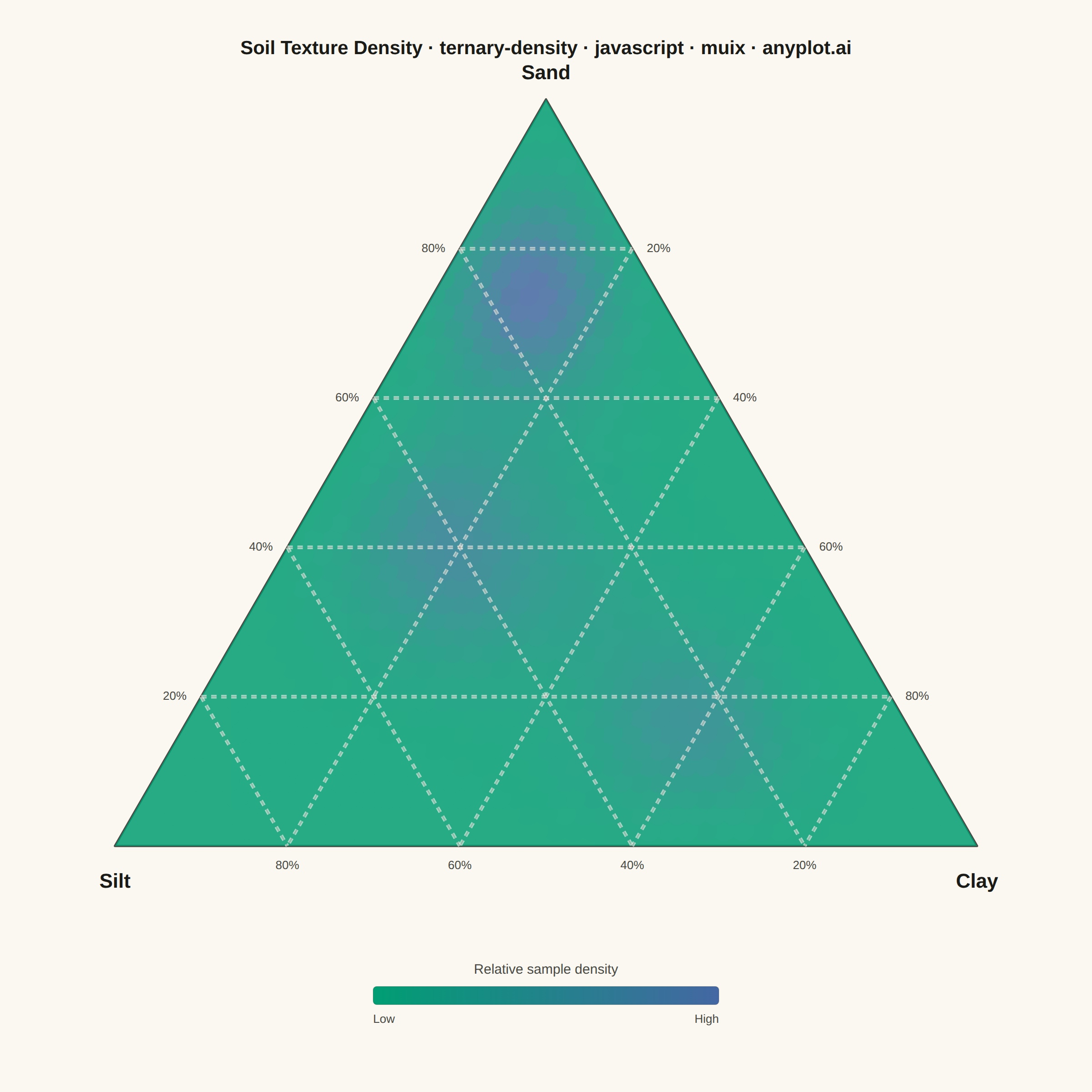
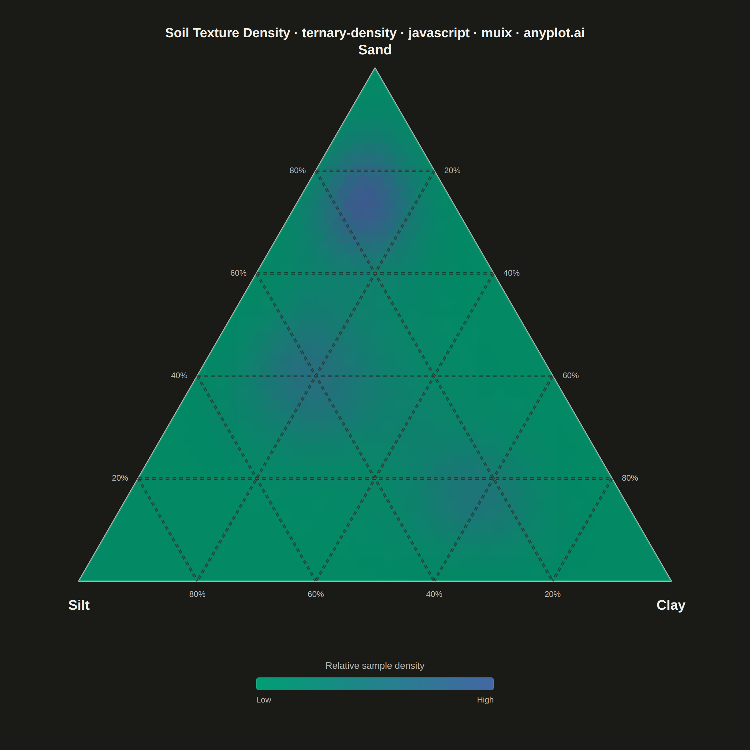
The same plot in 14 other libraries — JavaScript: Chart.js, D3.js, Apache ECharts, Highcharts; Python: Altair, Bokeh, lets-plot, Matplotlib, Plotly, plotnine, Pygal, Seaborn; R: ggplot2; Julia: Makie.jl. Compare all 15 side by side: Ternary Density Plot in Python, R, Julia and JavaScript.
A ternary density plot combines a three-component ternary diagram with kernel density estimation to visualize where compositional data concentrates. Instead of showing individual points, this visualization uses a heatmap overlay to reveal the underlying probability distribution of compositions, making it ideal for identifying clusters, modes, and patterns in large compositional datasets.
// anyplot.ai
// ternary-density: Ternary Density Plot
// Library: muix 7.29.1 | JavaScript 22.23.2
// Quality: 88/100 | Created: 2026-09-02
//# anyplot-orientation: square
// anyplot.ai
// ternary-density: Ternary Density Plot
// Library: MUI X Charts | React | Node 22
// License: @mui/x-charts — MIT (community). Pro/Premium are out of scope.
// Quality: pending | Created: 2026-09-02
import { ChartContainer } from "@mui/x-charts/ChartContainer";
import { ScatterPlot } from "@mui/x-charts/ScatterChart";
import { ChartsTooltip } from "@mui/x-charts/ChartsTooltip";
import { useXScale, useYScale, useDrawingArea } from "@mui/x-charts/hooks";

const t = window.ANYPLOT_TOKENS;
const SIZE = window.ANYPLOT_SIZE;
const TITLE =
  "Soil Texture Density · ternary-density · javascript · muix · anyplot.ai";
const FONT =
  '-apple-system, BlinkMacSystemFont, "Segoe UI", Roboto, Helvetica, Arial, sans-serif';

// --- Ternary <-> Cartesian projection ---------------------------------------
// Equilateral triangle: Sand (a) at the top apex, Silt (b) at bottom-left,
// Clay (c) at bottom-right — the classic USDA soil-texture layout. Only two
// degrees of freedom exist (a+b+c=1), so every composition maps to a unique
// point inside (or on) the triangle.
const SQRT3_2 = Math.sqrt(3) / 2;
function toXY(a, b, c) {
  const total = a + b + c;
  const aN = a / total;
  const cN = c / total;
  return { x: cN + aN / 2, y: SQRT3_2 * aN };
}
const VERTEX_TOP = toXY(1, 0, 0);
const VERTEX_LEFT = toXY(0, 1, 0);
const VERTEX_RIGHT = toXY(0, 0, 1);

// --- Data: sand/silt/clay soil samples (deterministic, Dirichlet-like) -----
// Three characteristic soil-texture clouds — sandy, loamy, and clay-rich —
// each a Dirichlet-distributed cluster around a representative composition.
// The clusters overlap in the middle of the simplex, giving the KDE surface
// below a realistic multi-modal shape instead of one tidy blob.
let seed = 20260902 >>> 0;
function rand() {
  seed = (1664525 * seed + 1013904223) >>> 0;
  return seed / 4294967296;
}
function erlang(k) {
  let s = 0;
  for (let i = 0; i < k; i++) s += -Math.log(rand() || 1e-9);
  return s;
}

const CLUSTERS = [
  { n: 190, shape: [19, 4, 3] }, // sandy soils — sand-dominant, tight cluster
  { n: 220, shape: [8, 8, 4] }, // loamy soils — the most common texture class
  { n: 170, shape: [4, 5, 11] }, // clay-rich soils — clay-dominant
];

const samplePoints = [];
for (const cluster of CLUSTERS) {
  for (let i = 0; i < cluster.n; i++) {
    const gSand = erlang(cluster.shape[0]);
    const gSilt = erlang(cluster.shape[1]);
    const gClay = erlang(cluster.shape[2]);
    const total = gSand + gSilt + gClay;
    samplePoints.push(toXY(gSand / total, gSilt / total, gClay / total));
  }
}

// --- Kernel density estimate over a triangular lattice ---------------------
// A Gaussian KDE evaluated on every lattice point of a barycentric grid
// (i + j + k = GRID_N) — the natural equal-spacing grid for a simplex, and
// what the scatter markers below render as a continuous-looking heatmap.
const GRID_N = 46;
const BANDWIDTH = 0.055;
const TWO_H2 = 2 * BANDWIDTH * BANDWIDTH;

const densityPoints = [];
const sandPct = [];
const siltPct = [];
const clayPct = [];
let maxDensity = 0;
for (let i = 0; i <= GRID_N; i++) {
  for (let j = 0; j <= GRID_N - i; j++) {
    const k = GRID_N - i - j;
    const { x, y } = toXY(i, j, k);
    let density = 0;
    for (let s = 0; s < samplePoints.length; s++) {
      const dx = x - samplePoints[s].x;
      const dy = y - samplePoints[s].y;
      density += Math.exp(-(dx * dx + dy * dy) / TWO_H2);
    }
    density /= samplePoints.length;
    if (density > maxDensity) maxDensity = density;
    densityPoints.push({ x, y, z: density, rawZ: density, id: `cell-${i}-${j}` });
    sandPct.push(Math.round((i / GRID_N) * 100));
    siltPct.push(Math.round((j / GRID_N) * 100));
    clayPct.push(Math.round((k / GRID_N) * 100));
  }
}

// Steepen the density -> color mapping with a gamma > 1: this pushes the
// broad low-density field further toward the green end of imprint_seq while
// leaving true peaks near the blue end, so the three clusters read as
// distinct hotspots instead of one uniform green wash. `rawZ` (linear,
// untouched) still drives the opacity mask below and the tooltip percentage.
const COLOR_GAMMA = 1.7;
for (const p of densityPoints) {
  p.z = Math.pow(p.rawZ / maxDensity, COLOR_GAMMA) * maxDensity;
}

// --- Reference grid: lines of constant composition, parallel to each edge --
const GRID_LEVELS = [0.2, 0.4, 0.6, 0.8];
const GRID_SEGMENTS = [];
for (const f of GRID_LEVELS) {
  GRID_SEGMENTS.push([toXY(f, 1 - f, 0), toXY(f, 0, 1 - f)]); // constant Sand
  GRID_SEGMENTS.push([toXY(1 - f, f, 0), toXY(0, f, 1 - f)]); // constant Silt
  GRID_SEGMENTS.push([toXY(1 - f, 0, f), toXY(0, 1 - f, f)]); // constant Clay
}
const TICK_LEVELS = [20, 40, 60, 80];
const LEFT_TICKS = TICK_LEVELS.map((pct) => ({
  pct,
  pos: toXY(pct / 100, 1 - pct / 100, 0),
}));
const BOTTOM_TICKS = TICK_LEVELS.map((pct) => ({
  pct,
  pos: toXY(0, pct / 100, 1 - pct / 100),
}));
const RIGHT_TICKS = TICK_LEVELS.map((pct) => ({
  pct,
  pos: toXY(1 - pct / 100, 0, pct / 100),
}));

// Domain padding around the [0,1] x [0, sqrt3/2] triangle. Equal x/y spans
// (1.216) keep the triangle equilateral on the square canvas — extra room
// above for the title, and generously below for vertex labels + the density
// legend, which both live outside the triangle itself.
const X_MIN = -0.108;
const X_MAX = 1.108;
const Y_MIN = -0.26;
const Y_MAX = 0.956;

function TriangleGrid() {
  const xs = useXScale();
  const ys = useYScale();
  return (
    <g>
      {GRID_SEGMENTS.map((seg, i) => (
        <line
          key={i}
          x1={xs(seg[0].x)}
          y1={ys(seg[0].y)}
          x2={xs(seg[1].x)}
          y2={ys(seg[1].y)}
          stroke={t.grid}
          strokeWidth={1.5}
          strokeDasharray="6 5"
        />
      ))}
      <path
        d={`M${xs(VERTEX_TOP.x)} ${ys(VERTEX_TOP.y)} L${xs(VERTEX_LEFT.x)} ${ys(VERTEX_LEFT.y)} L${xs(VERTEX_RIGHT.x)} ${ys(VERTEX_RIGHT.y)} Z`}
        fill="none"
        stroke={t.inkSoft}
        strokeWidth={2.5}
        strokeLinejoin="round"
      />
    </g>
  );
}

function DensityLayer() {
  const xs = useXScale();
  const ys = useYScale();
  const clipD = `M${xs(VERTEX_TOP.x)} ${ys(VERTEX_TOP.y)} L${xs(VERTEX_LEFT.x)} ${ys(VERTEX_LEFT.y)} L${xs(VERTEX_RIGHT.x)} ${ys(VERTEX_RIGHT.y)} Z`;
  return (
    <>
      <defs>
        <clipPath id="ternaryTriangleClip">
          <path d={clipD} />
        </clipPath>
      </defs>
      <g clipPath="url(#ternaryTriangleClip)" opacity={0.85}>
        <ScatterPlot />
      </g>
    </>
  );
}

// A second, higher-contrast pass of the reference grid drawn ON TOP of the
// density layer: a page-background-colored halo "cuts through" the density
// fill, then the actual dashed grid stroke reads over it — guaranteed
// visible everywhere (including the high-density peaks that fully occlude
// the beneath-the-density copy in TriangleGrid) in both themes.
function GridOverlay() {
  const xs = useXScale();
  const ys = useYScale();
  return (
    <g>
      {GRID_SEGMENTS.map((seg, i) => (
        <line
          key={`halo-${i}`}
          x1={xs(seg[0].x)}
          y1={ys(seg[0].y)}
          x2={xs(seg[1].x)}
          y2={ys(seg[1].y)}
          stroke={t.pageBg}
          strokeWidth={4}
          strokeOpacity={0.6}
          strokeDasharray="6 5"
        />
      ))}
      {GRID_SEGMENTS.map((seg, i) => (
        <line
          key={`line-${i}`}
          x1={xs(seg[0].x)}
          y1={ys(seg[0].y)}
          x2={xs(seg[1].x)}
          y2={ys(seg[1].y)}
          stroke={t.grid}
          strokeWidth={1.5}
          strokeDasharray="6 5"
        />
      ))}
    </g>
  );
}

function EdgeTicks() {
  const xs = useXScale();
  const ys = useYScale();
  const label = (tick, dx, dy, anchor) => (
    <text
      key={`${dx}-${dy}-${tick.pct}`}
      x={xs(tick.pos.x) + dx}
      y={ys(tick.pos.y) + dy}
      textAnchor={anchor}
      dominantBaseline="middle"
      fontFamily={FONT}
      fontSize={13}
      fill={t.inkSoft}
    >
      {tick.pct}%
    </text>
  );
  return (
    <g>
      {LEFT_TICKS.map((tk) => label(tk, -16, 0, "end"))}
      {BOTTOM_TICKS.map((tk) => label(tk, 0, 22, "middle"))}
      {RIGHT_TICKS.map((tk) => label(tk, 16, 0, "start"))}
    </g>
  );
}

function VertexLabels() {
  const xs = useXScale();
  const ys = useYScale();
  return (
    <g fontFamily={FONT} fontSize={22} fontWeight={700} fill={t.ink}>
      <text
        x={xs(VERTEX_TOP.x)}
        y={ys(VERTEX_TOP.y) - 22}
        textAnchor="middle"
        dominantBaseline="baseline"
      >
        Sand
      </text>
      <text
        x={xs(VERTEX_LEFT.x)}
        y={ys(VERTEX_LEFT.y) + 30}
        textAnchor="middle"
        dominantBaseline="hanging"
      >
        Silt
      </text>
      <text
        x={xs(VERTEX_RIGHT.x)}
        y={ys(VERTEX_RIGHT.y) + 30}
        textAnchor="middle"
        dominantBaseline="hanging"
      >
        Clay
      </text>
    </g>
  );
}

function DensityLegend() {
  const { left, top, width, height } = useDrawingArea();
  const barWidth = Math.min(380, width * 0.36);
  const barHeight = 20;
  const cx = left + width / 2;
  const barY = top + height - 92;
  const barX = cx - barWidth / 2;
  return (
    <g fontFamily={FONT}>
      <defs>
        <linearGradient id="ternaryDensityGradient" x1="0" x2="1" y1="0" y2="0">
          <stop offset="0%" stopColor={t.seq[0]} />
          <stop offset="100%" stopColor={t.seq[1]} />
        </linearGradient>
      </defs>
      <text
        x={cx}
        y={barY - 14}
        textAnchor="middle"
        fontSize={15}
        fill={t.inkSoft}
      >
        Relative sample density
      </text>
      <rect
        x={barX}
        y={barY}
        width={barWidth}
        height={barHeight}
        rx={4}
        fill="url(#ternaryDensityGradient)"
        stroke={t.ink}
        strokeOpacity={0.15}
      />
      <text
        x={barX}
        y={barY + barHeight + 20}
        textAnchor="start"
        fontSize={13}
        fill={t.inkSoft}
      >
        Low
      </text>
      <text
        x={barX + barWidth}
        y={barY + barHeight + 20}
        textAnchor="end"
        fontSize={13}
        fill={t.inkSoft}
      >
        High
      </text>
    </g>
  );
}

function Title() {
  const xs = useXScale();
  const ys = useYScale();
  const n = TITLE.length;
  const ratio = n > 67 ? 67 / n : 1.0;
  const fontSize = Math.max(15, Math.round(22 * ratio));
  return (
    <text
      x={xs((X_MIN + X_MAX) / 2)}
      y={ys(Y_MAX) + fontSize}
      textAnchor="middle"
      dominantBaseline="hanging"
      fontFamily={FONT}
      fontSize={fontSize}
      fontWeight={600}
      fill={t.ink}
    >
      {TITLE}
    </text>
  );
}

// --- Chart (default-exported component — the harness mounts it) -------------
export default function Chart() {
  return (
    <ChartContainer
      width={SIZE.width}
      height={SIZE.height}
      margin={{ top: 24, right: 24, bottom: 24, left: 24 }}
      series={[
        {
          type: "scatter",
          label: "Sample density",
          color: t.seq[0],
          markerSize: 13,
          data: densityPoints,
          valueFormatter: (_value, ctx) =>
            `Sand ${sandPct[ctx.dataIndex]}% · Silt ${siltPct[ctx.dataIndex]}% · Clay ${clayPct[ctx.dataIndex]}% — ${Math.round((densityPoints[ctx.dataIndex].rawZ / maxDensity) * 100)}% of peak density`,
        },
      ]}
      xAxis={[{ scaleType: "linear", min: X_MIN, max: X_MAX }]}
      yAxis={[{ scaleType: "linear", min: Y_MIN, max: Y_MAX }]}
      zAxis={[
        {
          id: "density",
          min: 0,
          max: maxDensity,
          colorMap: { type: "continuous", color: [t.seq[0], t.seq[1]] },
        },
      ]}
      skipAnimation
    >
      <TriangleGrid />
      <DensityLayer />
      <GridOverlay />
      <EdgeTicks />
      <VertexLabels />
      <DensityLegend />
      <Title />
      <ChartsTooltip trigger="item" />
    </ChartContainer>
  );
}
Runnable source as JSON, for any HTTP client: https://api.anyplot.ai/specs/ternary-density/muix/code. Any spec id and library id listed in llms-full.txt fit the same URL shape; every URL below is complete and callable.
{
  "spec_id": "ternary-density",
  "language": "javascript",
  "library": "muix",
  "page": "https://anyplot.ai/ternary-density/javascript/muix",
  "hub": "https://anyplot.ai/ternary-density",
  "code_json": "https://api.anyplot.ai/specs/ternary-density/muix/code",
  "spec_json": "https://api.anyplot.ai/specs/ternary-density",
  "render_light_png": "https://storage.googleapis.com/anyplot-images/plots/ternary-density/javascript/muix/plot-light.png",
  "render_dark_png": "https://storage.googleapis.com/anyplot-images/plots/ternary-density/javascript/muix/plot-dark.png",
  "interactive_light_html": "https://storage.googleapis.com/anyplot-images/plots/ternary-density/javascript/muix/plot-light.html",
  "interactive_dark_html": "https://storage.googleapis.com/anyplot-images/plots/ternary-density/javascript/muix/plot-dark.html",
  "quality_score": 88.0,
  "license": "MIT",
  "guide": "https://anyplot.ai/llms.txt"
}
Part of Ternary Density Plot on anyplot.ai.