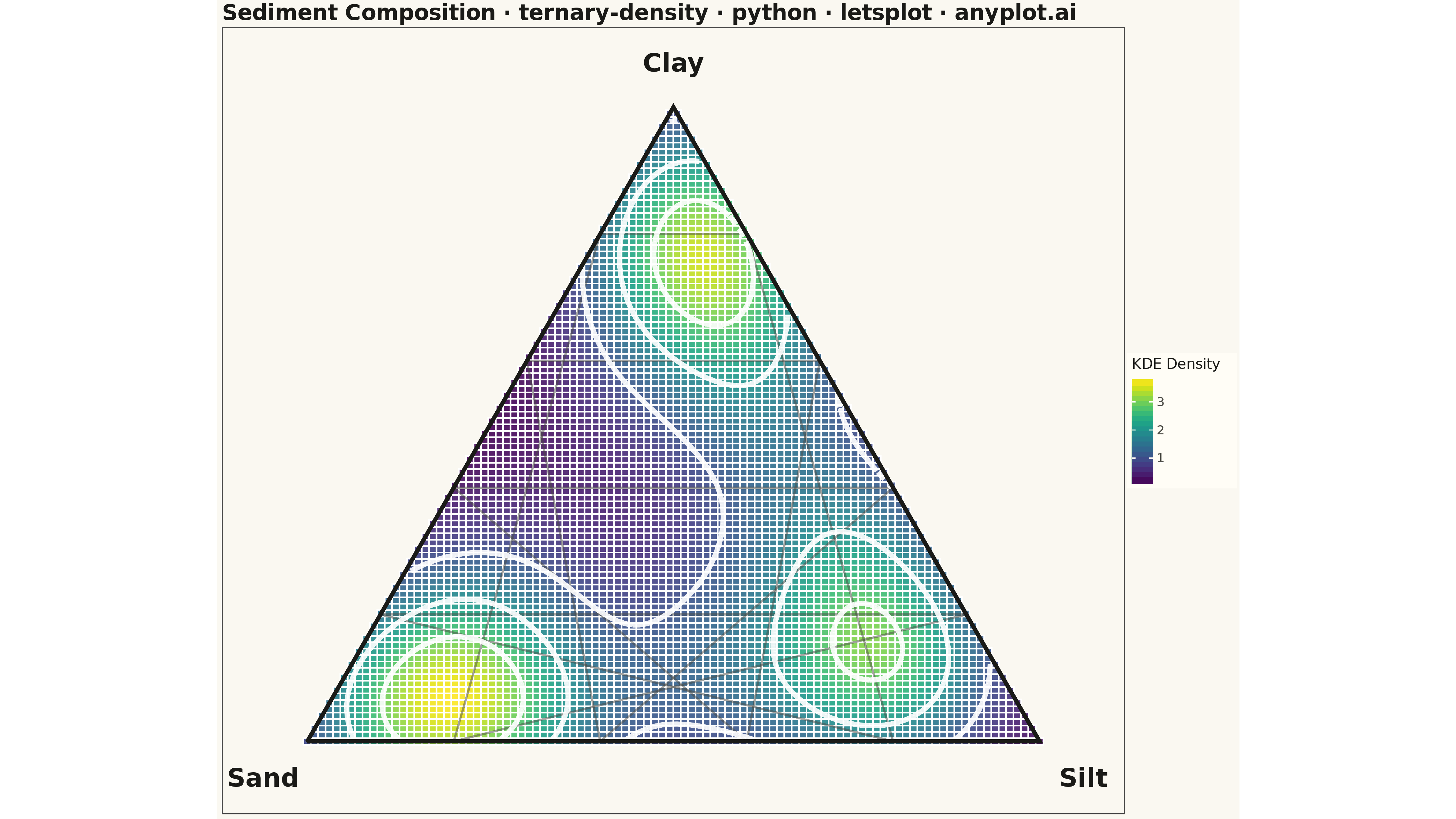
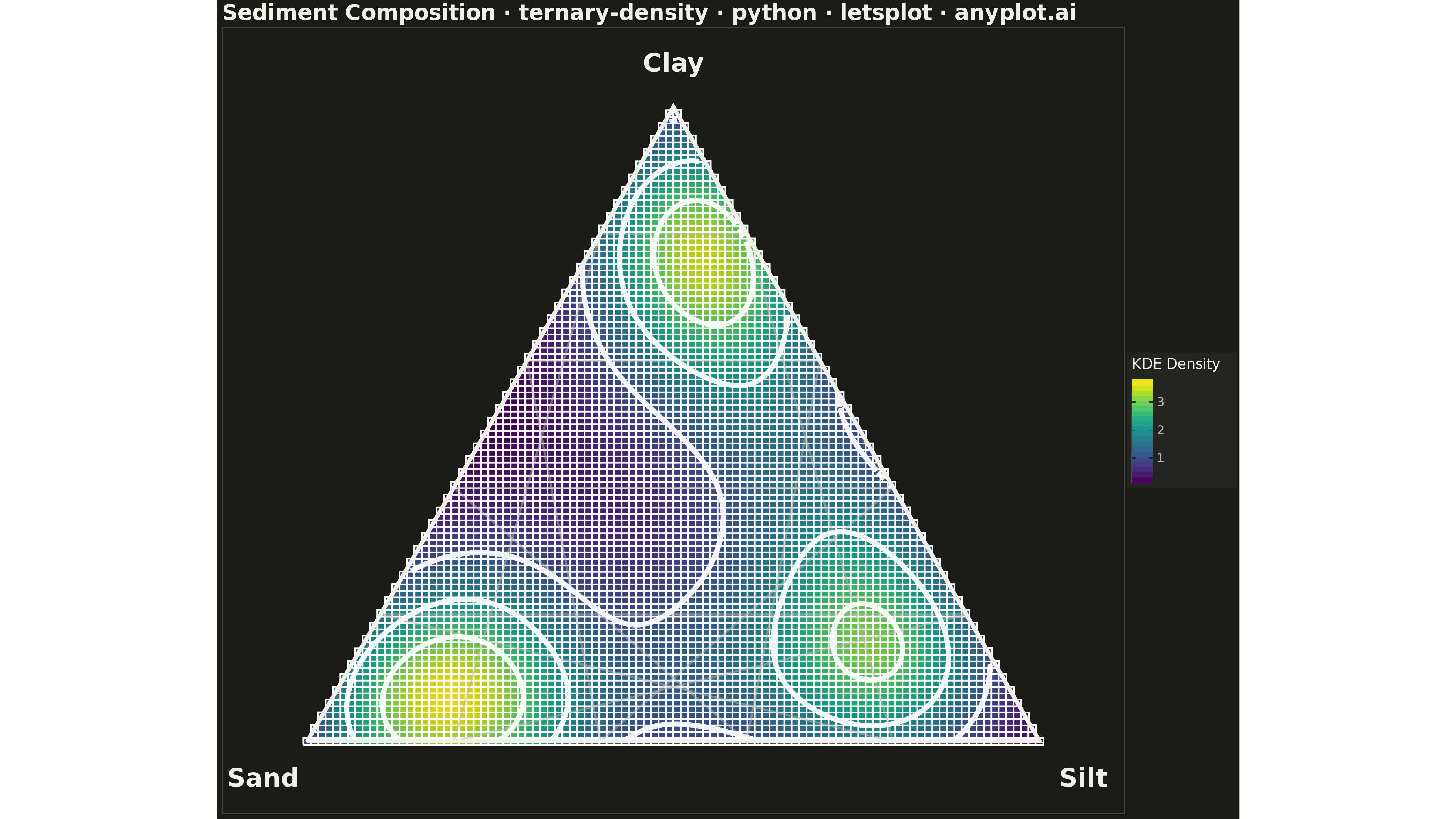
A ternary density plot combines a three-component ternary diagram with kernel density estimation to visualize where compositional data concentrates. Instead of showing individual points, this visualization uses a heatmap overlay to reveal the underlying probability distribution of compositions, making it ideal for identifying clusters, modes, and patterns in large compositional datasets.
""" anyplot.ai
ternary-density: Ternary Density Plot
Library: letsplot 4.9.0 | Python 3.13.13
Quality: 87/100 | Updated: 2026-05-19
"""

import os

import numpy as np
import pandas as pd
from lets_plot import (
    LetsPlot,
    aes,
    coord_fixed,
    element_blank,
    element_rect,
    element_text,
    geom_path,
    geom_point,
    geom_polygon,
    geom_segment,
    geom_text,
    ggplot,
    ggsave,
    ggsize,
    labs,
    layer_tooltips,
    scale_fill_viridis,
    theme,
)


LetsPlot.setup_html()

# Theme tokens
THEME = os.getenv("ANYPLOT_THEME", "light")
PAGE_BG = "#FAF8F1" if THEME == "light" else "#1A1A17"
ELEVATED_BG = "#FFFDF6" if THEME == "light" else "#242420"
INK = "#1A1A17" if THEME == "light" else "#F0EFE8"
INK_SOFT = "#4A4A44" if THEME == "light" else "#B8B7B0"

# Data — synthetic compositional data (sediment: sand/silt/clay)
np.random.seed(42)

# Three clusters via Dirichlet distribution
alpha1 = np.array([8, 2, 1])
comp1 = np.random.dirichlet(alpha1, 180) * 100

alpha2 = np.array([2, 7, 2])
comp2 = np.random.dirichlet(alpha2, 160) * 100

alpha3 = np.array([1, 2, 8])
comp3 = np.random.dirichlet(alpha3, 160) * 100

compositions = np.vstack([comp1, comp2, comp3])
sand = compositions[:, 0]
silt = compositions[:, 1]
clay = compositions[:, 2]

# Convert ternary to Cartesian coordinates
# bottom-left = Sand, bottom-right = Silt, top = Clay
total = sand + silt + clay
b_norm = silt / total
c_norm = clay / total

x_data = 0.5 * (2 * b_norm + c_norm)
y_data = (np.sqrt(3) / 2) * c_norm

# Density grid
grid_res = 100
x_grid = np.linspace(0, 1, grid_res)
y_grid = np.linspace(0, np.sqrt(3) / 2, grid_res)
X, Y = np.meshgrid(x_grid, y_grid)

# 2D Gaussian KDE (Scott's rule)
n = len(x_data)
bw = n ** (-1.0 / 6)
bw_x = np.std(x_data) * bw
bw_y = np.std(y_data) * bw

Z = np.zeros_like(X)
for i in range(n):
    dx = (X - x_data[i]) / bw_x
    dy = (Y - y_data[i]) / bw_y
    Z += np.exp(-0.5 * (dx**2 + dy**2))
Z /= n * 2 * np.pi * bw_x * bw_y

# Mask points outside the equilateral triangle
sqrt3 = np.sqrt(3)
mask = (Y >= 0) & (Y <= sqrt3 * X + 1e-6) & (Y <= sqrt3 * (1 - X) + 1e-6)

# Density polygons dataframe
polygon_data = []
poly_id = 0
dx = x_grid[1] - x_grid[0]
dy = y_grid[1] - y_grid[0]
overlap = 1.05

for i in range(grid_res):
    for j in range(grid_res):
        if mask[i, j] and Z[i, j] > 0:
            cx, cy = X[i, j], Y[i, j]
            hdx = dx * overlap / 2
            hdy = dy * overlap / 2
            corners_x = [cx - hdx, cx + hdx, cx + hdx, cx - hdx, cx - hdx]
            corners_y = [cy - hdy, cy - hdy, cy + hdy, cy + hdy, cy - hdy]
            for k in range(5):
                polygon_data.append({"x": corners_x[k], "y": corners_y[k], "density": Z[i, j], "id": poly_id})
            poly_id += 1

df_polygons = pd.DataFrame(polygon_data)

# Contour lines via marching squares at 25%, 50%, 75% density levels
z_masked = Z.copy()
z_masked[~mask] = 0
z_min, z_max = z_masked[mask].min(), z_masked[mask].max()
contour_levels = [z_min + (z_max - z_min) * p for p in [0.25, 0.5, 0.75]]

contour_data = []
for level in contour_levels:
    for i in range(grid_res - 1):
        for j in range(grid_res - 1):
            corners = [Z[i, j], Z[i, j + 1], Z[i + 1, j + 1], Z[i + 1, j]]
            corners_mask = [mask[i, j], mask[i, j + 1], mask[i + 1, j + 1], mask[i + 1, j]]
            if not all(corners_mask):
                continue
            above = [c >= level for c in corners]
            if all(above) or not any(above):
                continue
            x0, x1 = x_grid[j], x_grid[j + 1]
            y0, y1 = y_grid[i], y_grid[i + 1]
            pts = []
            if above[0] != above[1]:
                t = (level - corners[0]) / (corners[1] - corners[0] + 1e-10)
                pts.append((x0 + t * (x1 - x0), y0))
            if above[1] != above[2]:
                t = (level - corners[1]) / (corners[2] - corners[1] + 1e-10)
                pts.append((x1, y0 + t * (y1 - y0)))
            if above[2] != above[3]:
                t = (level - corners[2]) / (corners[3] - corners[2] + 1e-10)
                pts.append((x1 - t * (x1 - x0), y1))
            if above[3] != above[0]:
                t = (level - corners[3]) / (corners[0] - corners[3] + 1e-10)
                pts.append((x0, y1 - t * (y1 - y0)))
            if len(pts) == 2:
                contour_data.append({"x": pts[0][0], "y": pts[0][1], "xend": pts[1][0], "yend": pts[1][1]})

df_contours = pd.DataFrame(contour_data) if contour_data else pd.DataFrame(columns=["x", "y", "xend", "yend"])

# Triangle outline
tri_x = [0, 1, 0.5, 0]
tri_y = [0, 0, sqrt3 / 2, 0]
df_triangle = pd.DataFrame({"x": tri_x, "y": tri_y})

# Grid lines inside the triangle
grid_lines = []
for pct in [0.2, 0.4, 0.6, 0.8]:
    # Parallel to bottom edge (constant clay %)
    y_line = pct * sqrt3 / 2
    grid_lines.append({"x": pct / 2, "xend": 1 - pct / 2, "y": y_line, "yend": y_line})
    # Parallel to left edge (constant silt %)
    grid_lines.append({"x": pct, "xend": 1 - 0.5 * pct, "y": 0.0, "yend": pct * sqrt3 / 2})
    # Parallel to right edge (constant sand %)
    grid_lines.append({"x": 1 - pct, "xend": 0.5 * pct, "y": 0.0, "yend": pct * sqrt3 / 2})

df_grid = pd.DataFrame(grid_lines)

# Vertex labels
labels_data = pd.DataFrame(
    {"x": [-0.06, 1.06, 0.5], "y": [-0.05, -0.05, sqrt3 / 2 + 0.06], "label": ["Sand", "Silt", "Clay"]}
)

# Scatter data for interactive HTML tooltips showing composition at each point
df_scatter = pd.DataFrame(
    {"x": x_data, "y": y_data, "Sand": sand.round(1), "Silt": silt.round(1), "Clay": clay.round(1)}
)

# Plot
plot = (
    ggplot()
    + geom_polygon(aes(x="x", y="y", fill="density", group="id"), data=df_polygons, color=None, alpha=0.9)
    + scale_fill_viridis(name="KDE Density", option="viridis")
    + geom_segment(aes(x="x", y="y", xend="xend", yend="yend"), data=df_grid, color=INK_SOFT, size=1.0, alpha=0.5)
    + (
        geom_segment(
            aes(x="x", y="y", xend="xend", yend="yend"),
            data=df_contours,
            color="white",
            size=2.5,
            alpha=0.9,
            linetype="dashed",
        )
        if len(df_contours) > 0
        else geom_path(aes(x="x", y="y"), data=pd.DataFrame({"x": [], "y": []}))
    )
    + geom_path(aes(x="x", y="y"), data=df_triangle, color=INK, size=2.0)
    + geom_point(
        aes(x="x", y="y"),
        data=df_scatter,
        color="white",
        size=1,
        alpha=0.01,
        tooltips=layer_tooltips().line("Sand: @Sand%").line("Silt: @Silt%").line("Clay: @Clay%"),
    )
    + geom_text(aes(x="x", y="y", label="label"), data=labels_data, color=INK, size=14, fontface="bold")
    + labs(title="Sediment Composition · ternary-density · python · letsplot · anyplot.ai", x="", y="")
    + coord_fixed(ratio=1)
    + theme(
        plot_background=element_rect(fill=PAGE_BG, color=PAGE_BG),
        panel_background=element_rect(fill=PAGE_BG),
        panel_grid=element_blank(),
        axis_title=element_blank(),
        axis_text=element_blank(),
        axis_ticks=element_blank(),
        axis_line=element_blank(),
        plot_title=element_text(size=24, face="bold", color=INK),
        legend_background=element_rect(fill=ELEVATED_BG, color=INK_SOFT),
        legend_title=element_text(size=16, color=INK),
        legend_text=element_text(size=14, color=INK_SOFT),
    )
    + ggsize(1600, 900)
)

# Save
ggsave(plot, f"plot-{THEME}.png", path=".", scale=3)
ggsave(plot, f"plot-{THEME}.html", path=".")
Runnable source as JSON, for any HTTP client: https://api.anyplot.ai/specs/ternary-density/letsplot/code. Any spec id and library id listed in llms-full.txt fit the same URL shape; every URL below is complete and callable.
{
  "spec_id": "ternary-density",
  "language": "python",
  "library": "letsplot",
  "page": "https://anyplot.ai/ternary-density/python/letsplot",
  "hub": "https://anyplot.ai/ternary-density",
  "code_json": "https://api.anyplot.ai/specs/ternary-density/letsplot/code",
  "spec_json": "https://api.anyplot.ai/specs/ternary-density",
  "render_light_png": "https://storage.googleapis.com/anyplot-images/plots/ternary-density/python/letsplot/plot-light.png",
  "render_dark_png": "https://storage.googleapis.com/anyplot-images/plots/ternary-density/python/letsplot/plot-dark.png",
  "interactive_light_html": "https://storage.googleapis.com/anyplot-images/plots/ternary-density/python/letsplot/plot-light.html",
  "interactive_dark_html": "https://storage.googleapis.com/anyplot-images/plots/ternary-density/python/letsplot/plot-dark.html",
  "quality_score": 87.0,
  "license": "MIT",
  "guide": "https://anyplot.ai/llms.txt"
}
Part of Ternary Density Plot on anyplot.ai.