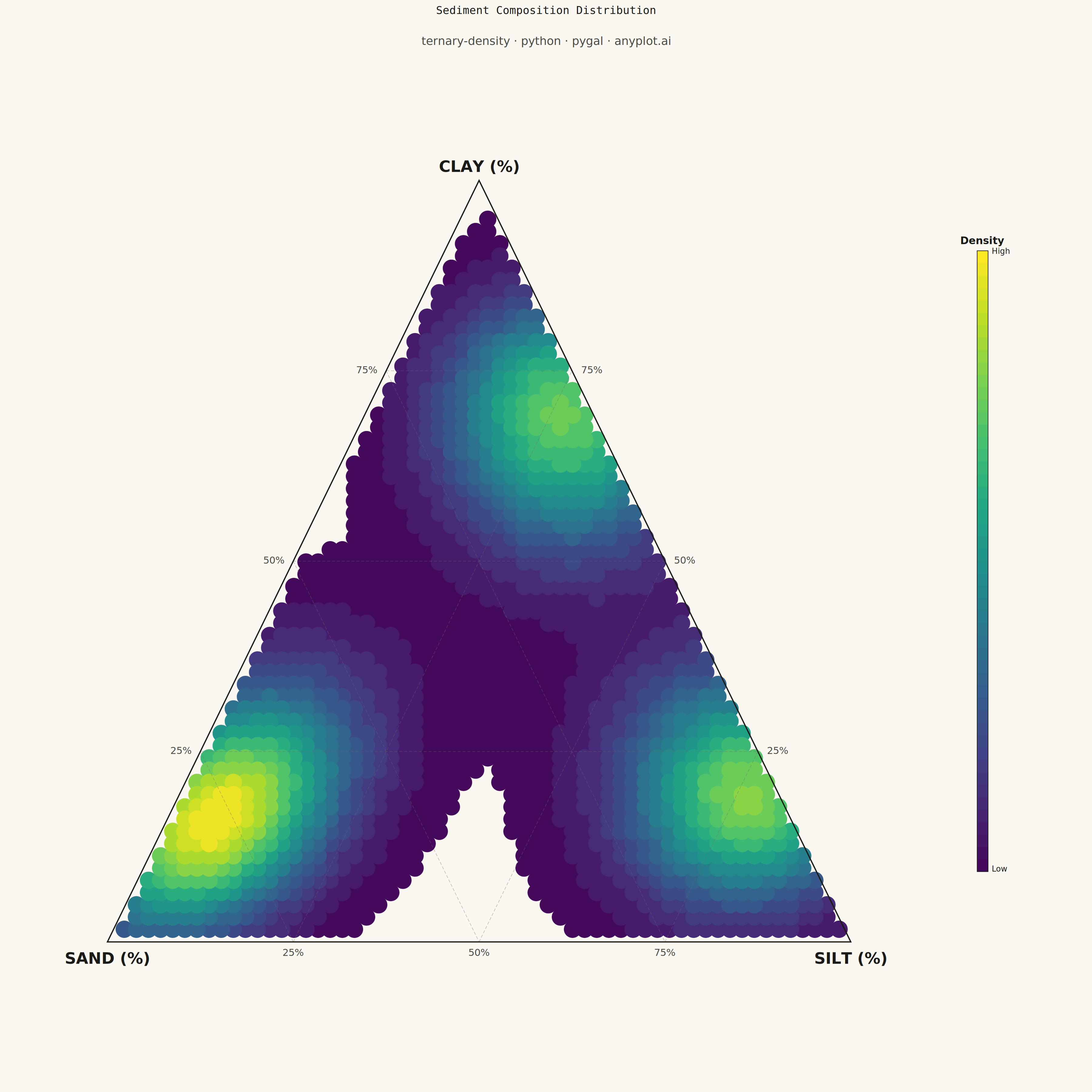
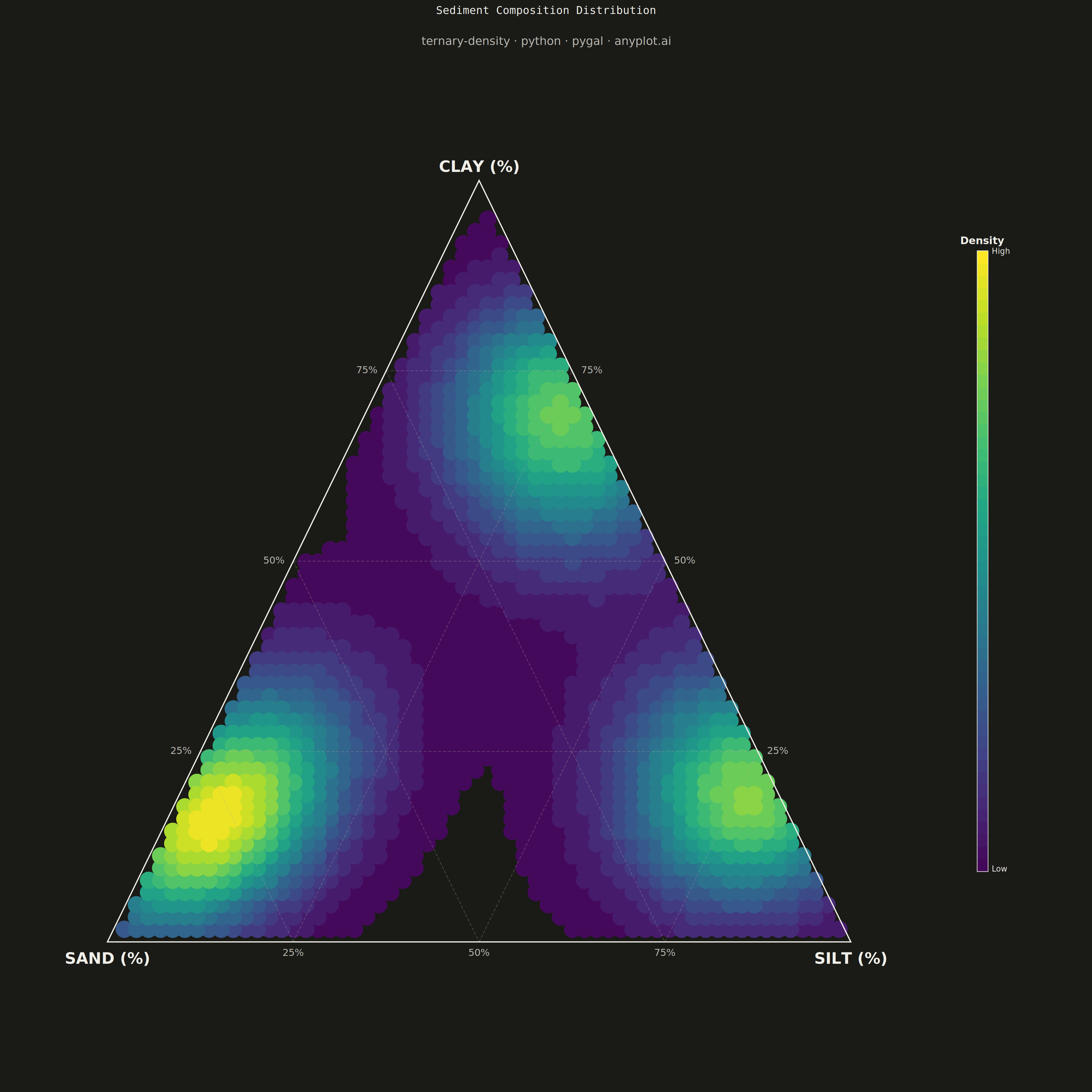
A ternary density plot combines a three-component ternary diagram with kernel density estimation to visualize where compositional data concentrates. Instead of showing individual points, this visualization uses a heatmap overlay to reveal the underlying probability distribution of compositions, making it ideal for identifying clusters, modes, and patterns in large compositional datasets.
""" anyplot.ai
ternary-density: Ternary Density Plot
Library: pygal 3.1.0 | Python 3.13.13
Quality: 81/100 | Updated: 2026-05-19
"""

import math
import os

import cairosvg
import numpy as np
from scipy.stats import gaussian_kde


# Theme tokens
THEME = os.getenv("ANYPLOT_THEME", "light")
PAGE_BG = "#FAF8F1" if THEME == "light" else "#1A1A17"
INK = "#1A1A17" if THEME == "light" else "#F0EFE8"
INK_SOFT = "#4A4A44" if THEME == "light" else "#B8B7B0"
INK_MUTED = "#6B6A63" if THEME == "light" else "#A8A79F"

H = math.sqrt(3) / 2

np.random.seed(42)

# Data — sediment composition clusters (sand/silt/clay)
n1 = 300
sand1 = np.random.beta(5, 2, n1) * 60 + 35
silt1 = np.random.beta(2, 3, n1) * (100 - sand1) * 0.6
clay1 = 100 - sand1 - silt1

n2 = 250
silt2 = np.random.beta(5, 2, n2) * 50 + 40
sand2 = np.random.beta(2, 4, n2) * (100 - silt2) * 0.5
clay2 = 100 - sand2 - silt2

n3 = 250
clay3 = np.random.beta(4, 2, n3) * 45 + 40
sand3 = np.random.beta(2, 5, n3) * (100 - clay3) * 0.4
silt3 = 100 - sand3 - clay3

sand = np.clip(np.concatenate([sand1, sand2, sand3]), 0, 100)
silt = np.clip(np.concatenate([silt1, silt2, silt3]), 0, 100)
clay = np.clip(np.concatenate([clay1, clay2, clay3]), 0, 100)
total_comp = sand + silt + clay
sand, silt, clay = sand / total_comp * 100, silt / total_comp * 100, clay / total_comp * 100

# Ternary → Cartesian (Top=Clay, Bottom-left=Sand, Bottom-right=Silt)
x_data = 0.5 * (2 * silt / 100 + clay / 100)
y_data = H * clay / 100

# Density grid
grid_res = 100
xi = np.linspace(0, 1, grid_res)
yi = np.linspace(0, H, grid_res)
Xi, Yi = np.meshgrid(xi, yi)

# Triangle mask
Ci = Yi / H
Bi = Xi - Ci / 2
mask = ((1 - Bi - Ci) >= -0.001) & (Bi >= -0.001) & (Ci >= -0.001)

# KDE via scipy (Silverman bandwidth)
kde = gaussian_kde(np.vstack([x_data, y_data]))
Z = kde(np.vstack([Xi.ravel(), Yi.ravel()])).reshape(Xi.shape)
Z = np.where(mask, Z, 0)
Z_norm = (Z - Z.min()) / (Z.max() - Z.min() + 1e-10)

# Viridis color table (11 waypoints, R/G/B ∈ [0,1])
viridis_table = np.array(
    [
        [0.267004, 0.004874, 0.329415],
        [0.282327, 0.140926, 0.457517],
        [0.253935, 0.265254, 0.529983],
        [0.206756, 0.371758, 0.553117],
        [0.163625, 0.471133, 0.558148],
        [0.127568, 0.566949, 0.550556],
        [0.134692, 0.658636, 0.517649],
        [0.266941, 0.748751, 0.440573],
        [0.477504, 0.821444, 0.318195],
        [0.741388, 0.873449, 0.149561],
        [0.993248, 0.906157, 0.143936],
    ]
)

# Vectorized viridis color interpolation for all grid cells
v_idx = np.minimum((Z_norm * 10).astype(int), 9)
v_frac = Z_norm * 10 - v_idx.astype(float)
cell_r = viridis_table[v_idx, 0] * (1 - v_frac) + viridis_table[v_idx + 1, 0] * v_frac
cell_g = viridis_table[v_idx, 1] * (1 - v_frac) + viridis_table[v_idx + 1, 1] * v_frac
cell_b = viridis_table[v_idx, 2] * (1 - v_frac) + viridis_table[v_idx + 1, 2] * v_frac

# SVG canvas dimensions and coordinate mapping
chart_width = 3600
chart_height = 3600
margin = 200
plot_size = chart_width - 2 * margin
x_min, x_max = -0.12, 1.12
y_min, y_max = -0.15, H + 0.15
x_range = x_max - x_min
y_range = y_max - y_min

# Precompute pixel positions for density cell centers
cs_x = xi[1] - xi[0]
cs_y = yi[1] - yi[0]
px_c = margin + (xi[:-1] + cs_x / 2 - x_min) / x_range * plot_size
py_c = margin + (y_max - (yi[:-1] + cs_y / 2)) / y_range * plot_size
pw = cs_x / x_range * plot_size * 1.1
ph = cs_y / y_range * plot_size * 1.1

# Density heatmap
density_parts = ['<g id="density-layer" opacity="0.85">\n']
for i in range(grid_res - 1):
    for j in range(grid_res - 1):
        if mask[i, j] and Z_norm[i, j] > 0.05:
            r, g, b = int(cell_r[i, j] * 255), int(cell_g[i, j] * 255), int(cell_b[i, j] * 255)
            density_parts.append(
                f'  <rect x="{px_c[j] - pw / 2:.1f}" y="{py_c[i] - ph / 2:.1f}" width="{pw:.1f}" height="{ph:.1f}" fill="rgb({r},{g},{b})" />\n'
            )
density_parts.append("</g>\n")
density_svg = "".join(density_parts)

# Contour circles at density levels
contour_parts = [f'<g id="contour-lines" stroke="{PAGE_BG}" stroke-width="1.5" fill="none">\n']
for level in [0.2, 0.4, 0.6, 0.8]:
    thresh = Z_norm >= level
    for i in range(1, grid_res - 1):
        for j in range(1, grid_res - 1):
            if (
                thresh[i, j]
                and mask[i, j]
                and not all([thresh[i - 1, j], thresh[i + 1, j], thresh[i, j - 1], thresh[i, j + 1]])
            ):
                cx = margin + (xi[j] - x_min) / x_range * plot_size
                cy = margin + (y_max - yi[i]) / y_range * plot_size
                contour_parts.append(f'  <circle cx="{cx:.1f}" cy="{cy:.1f}" r="3" opacity="0.6" />\n')
contour_parts.append("</g>\n")
contour_svg = "".join(contour_parts)

# Triangle vertex pixel coordinates
vx_sand = margin + (0.0 - x_min) / x_range * plot_size
vy_sand = margin + (y_max - 0.0) / y_range * plot_size
vx_silt = margin + (1.0 - x_min) / x_range * plot_size
vy_silt = margin + (y_max - 0.0) / y_range * plot_size
vx_clay = margin + (0.5 - x_min) / x_range * plot_size
vy_clay = margin + (y_max - H) / y_range * plot_size

triangle_svg = f'<polygon points="{vx_sand:.1f},{vy_sand:.1f} {vx_silt:.1f},{vy_silt:.1f} {vx_clay:.1f},{vy_clay:.1f}" fill="none" stroke="{INK}" stroke-width="4" />'

# Grid lines at 25%, 50%, 75% (sparser spacing for cleaner readability)
grid_parts = [f'<g id="grid-lines" stroke="{INK_MUTED}" stroke-width="1.5" stroke-dasharray="10,6" opacity="0.5">\n']
for pct in [0.25, 0.50, 0.75]:
    # Constant clay lines: from (sand=1-pct, silt=0, clay=pct) to (sand=0, silt=1-pct, clay=pct)
    x1, y1 = 0.5 * pct, H * pct
    x2, y2 = 0.5 * (2 - pct), H * pct
    grid_parts.append(
        f'  <line x1="{margin + (x1 - x_min) / x_range * plot_size:.1f}" y1="{margin + (y_max - y1) / y_range * plot_size:.1f}" x2="{margin + (x2 - x_min) / x_range * plot_size:.1f}" y2="{margin + (y_max - y2) / y_range * plot_size:.1f}" />\n'
    )
    # Constant silt lines: from (sand=1-pct, silt=pct, clay=0) to (sand=0, silt=pct, clay=1-pct)
    x1, y1 = pct, 0.0
    x2, y2 = 0.5 * (pct + 1), H * (1 - pct)
    grid_parts.append(
        f'  <line x1="{margin + (x1 - x_min) / x_range * plot_size:.1f}" y1="{margin + (y_max - y1) / y_range * plot_size:.1f}" x2="{margin + (x2 - x_min) / x_range * plot_size:.1f}" y2="{margin + (y_max - y2) / y_range * plot_size:.1f}" />\n'
    )
    # Constant sand lines: from (sand=pct, silt=0, clay=1-pct) to (sand=pct, silt=1-pct, clay=0)
    x1, y1 = 0.5 * (1 - pct), H * (1 - pct)
    x2, y2 = 1 - pct, 0.0
    grid_parts.append(
        f'  <line x1="{margin + (x1 - x_min) / x_range * plot_size:.1f}" y1="{margin + (y_max - y1) / y_range * plot_size:.1f}" x2="{margin + (x2 - x_min) / x_range * plot_size:.1f}" y2="{margin + (y_max - y2) / y_range * plot_size:.1f}" />\n'
    )
grid_parts.append("</g>\n")
grid_svg = "".join(grid_parts)

# Vertex labels with % unit indicator
label_svg = f'''<g id="vertex-labels" font-family="sans-serif" font-weight="bold" fill="{INK}">
  <text x="{vx_sand - 30:.1f}" y="{vy_sand + 70:.1f}" font-size="56" text-anchor="middle">SAND (%)</text>
  <text x="{vx_silt + 30:.1f}" y="{vy_silt + 70:.1f}" font-size="56" text-anchor="middle">SILT (%)</text>
  <text x="{vx_clay:.1f}" y="{vy_clay - 40:.1f}" font-size="56" text-anchor="middle">CLAY (%)</text>
</g>
'''

# Percentage labels along edges at 25%, 50%, 75%
pct_parts = [f'<g id="pct-labels" font-family="sans-serif" font-size="36" fill="{INK_SOFT}">\n']
for pct in [25, 50, 75]:
    frac = pct / 100
    # Bottom edge (Sand-Silt axis): silt varies
    bx, by = frac, 0.0
    bpx = margin + (bx - x_min) / x_range * plot_size
    bpy = margin + (y_max - by) / y_range * plot_size
    pct_parts.append(f'  <text x="{bpx:.1f}" y="{bpy + 45:.1f}" text-anchor="middle">{pct}%</text>\n')
    # Left edge (Sand-Clay axis): clay varies
    lx, ly = 0.5 * frac, H * frac
    lpx = margin + (lx - x_min) / x_range * plot_size
    lpy = margin + (y_max - ly) / y_range * plot_size
    pct_parts.append(f'  <text x="{lpx - 35:.1f}" y="{lpy + 10:.1f}" text-anchor="end">{pct}%</text>\n')
    # Right edge (Silt-Clay axis): clay varies
    rx, ry = 0.5 * (2 - frac), H * frac
    rpx = margin + (rx - x_min) / x_range * plot_size
    rpy = margin + (y_max - ry) / y_range * plot_size
    pct_parts.append(f'  <text x="{rpx + 35:.1f}" y="{rpy + 10:.1f}" text-anchor="start">{pct}%</text>\n')
pct_parts.append("</g>\n")
pct_svg = "".join(pct_parts)

# Colorbar
cbar_x = chart_width - margin + 40
cbar_y = margin + 200
cbar_w = 40
cbar_h = plot_size - 400

cbar_parts = [
    '<g id="colorbar">\n',
    f'  <text x="{cbar_x + cbar_w / 2:.1f}" y="{cbar_y - 30:.1f}" font-family="sans-serif" font-size="44" font-weight="bold" text-anchor="middle" fill="{INK}">Density</text>\n',
]
n_steps = 50
for i in range(n_steps):
    val = 1 - i / n_steps
    vi = min(int(val * 10), 9)
    vf = val * 10 - vi
    cr = int((viridis_table[vi, 0] * (1 - vf) + viridis_table[vi + 1, 0] * vf) * 255)
    cg = int((viridis_table[vi, 1] * (1 - vf) + viridis_table[vi + 1, 1] * vf) * 255)
    cb = int((viridis_table[vi, 2] * (1 - vf) + viridis_table[vi + 1, 2] * vf) * 255)
    cy = cbar_y + i / n_steps * cbar_h
    ch = cbar_h / n_steps + 1
    cbar_parts.append(
        f'  <rect x="{cbar_x:.1f}" y="{cy:.1f}" width="{cbar_w:.1f}" height="{ch:.1f}" fill="rgb({cr},{cg},{cb})" />\n'
    )
cbar_parts += [
    f'  <rect x="{cbar_x:.1f}" y="{cbar_y:.1f}" width="{cbar_w:.1f}" height="{cbar_h:.1f}" fill="none" stroke="{INK}" stroke-width="2" />\n',
    f'  <text x="{cbar_x + cbar_w + 15:.1f}" y="{cbar_y + 15:.1f}" font-family="sans-serif" font-size="32" fill="{INK}">High</text>\n',
    f'  <text x="{cbar_x + cbar_w + 15:.1f}" y="{cbar_y + cbar_h + 5:.1f}" font-family="sans-serif" font-size="32" fill="{INK}">Low</text>\n',
    "</g>\n",
]
colorbar_svg = "".join(cbar_parts)

# Title
title_svg = f'''<g id="title">
  <text x="{chart_width / 2:.1f}" y="100" font-family="sans-serif" font-size="72" font-weight="bold" text-anchor="middle" fill="{INK}">Sediment Composition Distribution</text>
  <text x="{chart_width / 2:.1f}" y="160" font-family="sans-serif" font-size="48" text-anchor="middle" fill="{INK_SOFT}">ternary-density · python · pygal · anyplot.ai</text>
</g>
'''

# Clip path for density layer
clip_svg = f'''<defs>
  <clipPath id="tri-clip">
    <polygon points="{vx_sand:.1f},{vy_sand:.1f} {vx_silt:.1f},{vy_silt:.1f} {vx_clay:.1f},{vy_clay:.1f}" />
  </clipPath>
</defs>'''

# Assemble SVG
svg = f"""<?xml version="1.0" encoding="UTF-8"?>
<svg xmlns="http://www.w3.org/2000/svg" width="{chart_width}" height="{chart_height}" viewBox="0 0 {chart_width} {chart_height}">
  <rect width="100%" height="100%" fill="{PAGE_BG}" />
  {clip_svg}
  {title_svg}
  <g clip-path="url(#tri-clip)">
    {density_svg}
    {contour_svg}
  </g>
  {grid_svg}
  <g>{triangle_svg}</g>
  {label_svg}
  {pct_svg}
  {colorbar_svg}
</svg>"""

# Save HTML and PNG (theme-suffixed)
with open(f"plot-{THEME}.html", "w") as f:
    f.write(svg)

cairosvg.svg2png(bytestring=svg.encode("utf-8"), write_to=f"plot-{THEME}.png")
Runnable source as JSON, for any HTTP client: https://api.anyplot.ai/specs/ternary-density/pygal/code. Any spec id and library id listed in llms-full.txt fit the same URL shape; every URL below is complete and callable.
{
  "spec_id": "ternary-density",
  "language": "python",
  "library": "pygal",
  "page": "https://anyplot.ai/ternary-density/python/pygal",
  "hub": "https://anyplot.ai/ternary-density",
  "code_json": "https://api.anyplot.ai/specs/ternary-density/pygal/code",
  "spec_json": "https://api.anyplot.ai/specs/ternary-density",
  "render_light_png": "https://storage.googleapis.com/anyplot-images/plots/ternary-density/python/pygal/plot-light.png",
  "render_dark_png": "https://storage.googleapis.com/anyplot-images/plots/ternary-density/python/pygal/plot-dark.png",
  "interactive_light_html": "https://storage.googleapis.com/anyplot-images/plots/ternary-density/python/pygal/plot-light.html",
  "interactive_dark_html": "https://storage.googleapis.com/anyplot-images/plots/ternary-density/python/pygal/plot-dark.html",
  "quality_score": 81.0,
  "license": "MIT",
  "guide": "https://anyplot.ai/llms.txt"
}
Part of Ternary Density Plot on anyplot.ai.