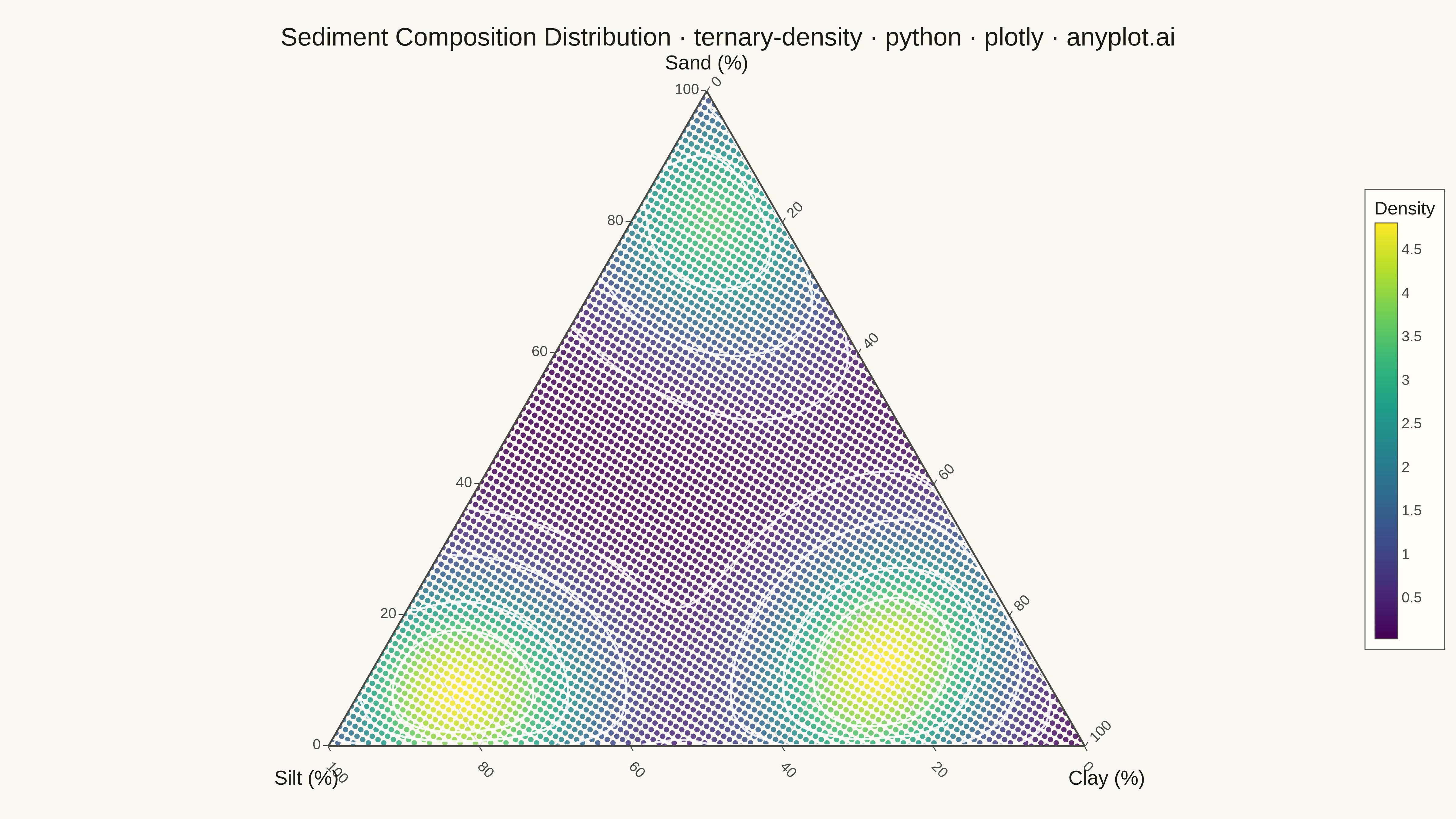
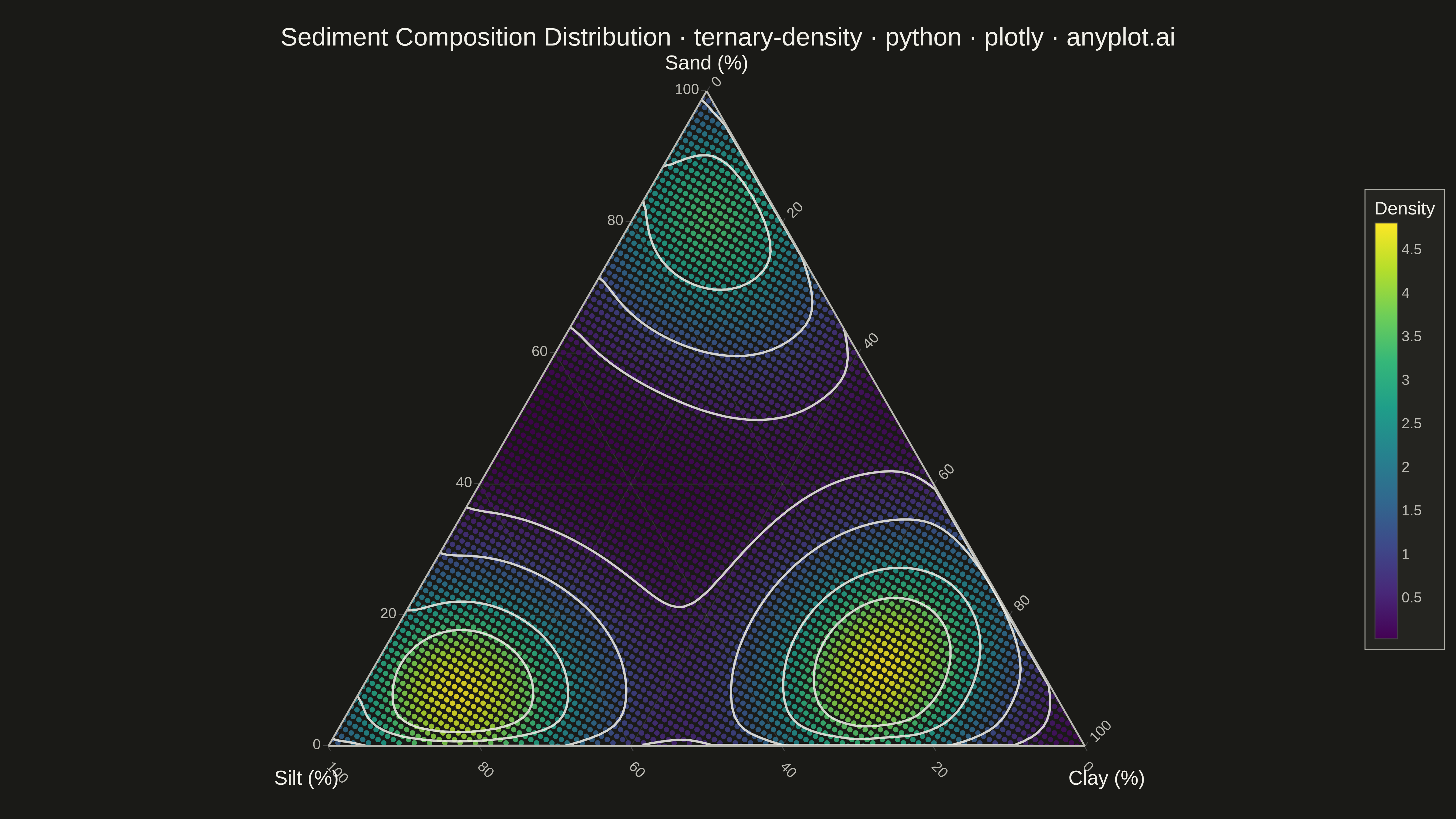
A ternary density plot combines a three-component ternary diagram with kernel density estimation to visualize where compositional data concentrates. Instead of showing individual points, this visualization uses a heatmap overlay to reveal the underlying probability distribution of compositions, making it ideal for identifying clusters, modes, and patterns in large compositional datasets.
""" anyplot.ai
ternary-density: Ternary Density Plot
Library: plotly 6.7.0 | Python 3.13.13
Quality: 91/100 | Updated: 2026-05-19
"""

import os
import sys


# Remove the script directory from sys.path so that sibling implementations
# (e.g. matplotlib.py) do not shadow installed packages.
_script_dir = os.path.dirname(os.path.abspath(__file__))
sys.path = [p for p in sys.path if os.path.abspath(p or os.getcwd()) != _script_dir]

import matplotlib


matplotlib.use("Agg")
import matplotlib.pyplot as plt
import numpy as np
import plotly.graph_objects as go
from scipy import ndimage
from scipy.stats import gaussian_kde


# Theme tokens
THEME = os.getenv("ANYPLOT_THEME", "light")
PAGE_BG = "#FAF8F1" if THEME == "light" else "#1A1A17"
ELEVATED_BG = "#FFFDF6" if THEME == "light" else "#242420"
INK = "#1A1A17" if THEME == "light" else "#F0EFE8"
INK_SOFT = "#4A4A44" if THEME == "light" else "#B8B7B0"
GRID = "rgba(26,26,23,0.12)" if THEME == "light" else "rgba(240,239,232,0.12)"

# Data — synthetic sediment composition (sand/silt/clay)
np.random.seed(42)
n_samples = 500

# Cluster 1: Sand-dominant samples (beaches/river channels)
cluster1_a = np.random.beta(8, 2, n_samples // 3) * 70 + 25
cluster1_b = np.random.beta(2, 5, n_samples // 3) * 40
cluster1_c = 100 - cluster1_a - cluster1_b
mask1 = cluster1_c >= 0
cluster1_a, cluster1_b, cluster1_c = cluster1_a[mask1], cluster1_b[mask1], cluster1_c[mask1]

# Cluster 2: Silt-dominant samples (floodplains/estuaries)
cluster2_b = np.random.beta(7, 2, n_samples // 3) * 55 + 35
cluster2_a = np.random.beta(2, 5, n_samples // 3) * 30
cluster2_c = 100 - cluster2_a - cluster2_b
mask2 = cluster2_c >= 0
cluster2_a, cluster2_b, cluster2_c = cluster2_a[mask2], cluster2_b[mask2], cluster2_c[mask2]

# Cluster 3: Clay-dominant mixed samples (deep lake sediments)
cluster3_c = np.random.beta(6, 2, n_samples // 3) * 50 + 30
cluster3_a = np.random.beta(2, 4, n_samples // 3) * 35
cluster3_b = 100 - cluster3_a - cluster3_c
mask3 = cluster3_b >= 0
cluster3_a, cluster3_b, cluster3_c = cluster3_a[mask3], cluster3_b[mask3], cluster3_c[mask3]

# Combine clusters
sand = np.concatenate([cluster1_a, cluster2_a, cluster3_a])
silt = np.concatenate([cluster1_b, cluster2_b, cluster3_b])
clay = np.concatenate([cluster1_c, cluster2_c, cluster3_c])

# Normalize to sum = 100
total = sand + silt + clay
sand = sand / total * 100
silt = silt / total * 100
clay = clay / total * 100

# Convert ternary → Cartesian for KDE
x_cart = 0.5 * (2 * silt + clay) / 100
y_cart = (np.sqrt(3) / 2) * clay / 100

# 2D kernel density estimation
coords = np.vstack([x_cart, y_cart])
kde = gaussian_kde(coords, bw_method="scott")

# Evaluation grid (Cartesian space)
grid_size = 100
x_grid = np.linspace(0, 1, grid_size)
y_grid = np.linspace(0, np.sqrt(3) / 2, grid_size)
xx, yy = np.meshgrid(x_grid, y_grid)
grid_coords = np.vstack([xx.ravel(), yy.ravel()])

density = kde(grid_coords).reshape(xx.shape)

# Mask outside the ternary triangle
inside_triangle = (yy >= 0) & (yy <= np.sqrt(3) * xx) & (yy <= np.sqrt(3) * (1 - xx))
density[~inside_triangle] = np.nan

# Back to ternary coordinates for plotting
clay_grid = yy * (2 / np.sqrt(3)) * 100
silt_grid = (xx - clay_grid / 200) * 100
sand_grid = 100 - silt_grid - clay_grid

# Plot
fig = go.Figure()

# Density layer — Viridis-colored scatter markers
valid_mask = inside_triangle & ~np.isnan(density)
a_flat = sand_grid[valid_mask]
b_flat = silt_grid[valid_mask]
c_flat = clay_grid[valid_mask]
d_flat = density[valid_mask]

fig.add_trace(
    go.Scatterternary(
        a=a_flat,
        b=b_flat,
        c=c_flat,
        mode="markers",
        marker={
            "size": 6,
            "color": d_flat,
            "colorscale": "Viridis",
            "showscale": True,
            "colorbar": {
                "title": {"text": "Density", "font": {"size": 20, "color": INK}},
                "tickfont": {"size": 16, "color": INK_SOFT},
                "len": 0.7,
                "thickness": 25,
                "x": 1.02,
                "bgcolor": ELEVATED_BG,
                "bordercolor": INK_SOFT,
                "borderwidth": 1,
            },
            "opacity": 0.85,
        },
        hovertemplate="Sand: %{a:.1f}%<br>Silt: %{b:.1f}%<br>Clay: %{c:.1f}%<extra></extra>",
        showlegend=False,
    )
)

# Smooth density for clean contour extraction
density_filled = density.copy()
density_filled[np.isnan(density_filled)] = 0
smoothed = ndimage.gaussian_filter(density_filled, sigma=2)

# Contour levels from smoothed valid region
smoothed_valid_vals = smoothed[inside_triangle]
contour_levels = np.percentile(smoothed_valid_vals[smoothed_valid_vals > 0], [25, 50, 75, 90])

# Extract smooth contour paths via matplotlib (data extraction only, no display)
fig_tmp, ax_tmp = plt.subplots()
CS = ax_tmp.contour(xx, yy, smoothed, levels=contour_levels)
plt.close(fig_tmp)

contour_color = "rgba(255,255,255,0.85)" if THEME == "light" else "rgba(240,239,232,0.85)"
for segs in CS.allsegs:
    for seg in segs:
        if len(seg) < 5:
            continue
        x_c, y_c = seg[:, 0], seg[:, 1]
        # Cartesian → ternary
        clay_c = y_c * (2 / np.sqrt(3)) * 100
        silt_c = (x_c - clay_c / 200) * 100
        sand_c = 100 - silt_c - clay_c
        # Filter to valid ternary region
        valid = (sand_c >= 0) & (silt_c >= 0) & (clay_c >= 0)
        if valid.sum() > 5:
            fig.add_trace(
                go.Scatterternary(
                    a=sand_c[valid],
                    b=silt_c[valid],
                    c=clay_c[valid],
                    mode="lines",
                    line={"color": contour_color, "width": 2.5},
                    hoverinfo="skip",
                    showlegend=False,
                )
            )

# Style
fig.update_layout(
    title={
        "text": "Sediment Composition Distribution · ternary-density · python · plotly · anyplot.ai",
        "font": {"size": 28, "color": INK},
        "x": 0.5,
        "xanchor": "center",
    },
    paper_bgcolor=PAGE_BG,
    plot_bgcolor=PAGE_BG,
    font={"color": INK},
    ternary={
        "sum": 100,
        "bgcolor": PAGE_BG,
        "aaxis": {
            "title": {"text": "Sand (%)", "font": {"size": 22, "color": INK}},
            "tickfont": {"size": 16, "color": INK_SOFT},
            "tickangle": 0,
            "dtick": 20,
            "gridcolor": GRID,
            "linecolor": INK_SOFT,
            "linewidth": 2,
        },
        "baxis": {
            "title": {"text": "Silt (%)", "font": {"size": 22, "color": INK}},
            "tickfont": {"size": 16, "color": INK_SOFT},
            "tickangle": 45,
            "dtick": 20,
            "gridcolor": GRID,
            "linecolor": INK_SOFT,
            "linewidth": 2,
        },
        "caxis": {
            "title": {"text": "Clay (%)", "font": {"size": 22, "color": INK}},
            "tickfont": {"size": 16, "color": INK_SOFT},
            "tickangle": -45,
            "dtick": 20,
            "gridcolor": GRID,
            "linecolor": INK_SOFT,
            "linewidth": 2,
        },
    },
    template="none",
    margin={"l": 80, "r": 120, "t": 100, "b": 80},
)

# Save
fig.write_image(f"plot-{THEME}.png", width=1600, height=900, scale=3)
fig.write_html(f"plot-{THEME}.html", include_plotlyjs="cdn")
Runnable source as JSON, for any HTTP client: https://api.anyplot.ai/specs/ternary-density/plotly/code. Any spec id and library id listed in llms-full.txt fit the same URL shape; every URL below is complete and callable.
{
  "spec_id": "ternary-density",
  "language": "python",
  "library": "plotly",
  "page": "https://anyplot.ai/ternary-density/python/plotly",
  "hub": "https://anyplot.ai/ternary-density",
  "code_json": "https://api.anyplot.ai/specs/ternary-density/plotly/code",
  "spec_json": "https://api.anyplot.ai/specs/ternary-density",
  "render_light_png": "https://storage.googleapis.com/anyplot-images/plots/ternary-density/python/plotly/plot-light.png",
  "render_dark_png": "https://storage.googleapis.com/anyplot-images/plots/ternary-density/python/plotly/plot-dark.png",
  "interactive_light_html": "https://storage.googleapis.com/anyplot-images/plots/ternary-density/python/plotly/plot-light.html",
  "interactive_dark_html": "https://storage.googleapis.com/anyplot-images/plots/ternary-density/python/plotly/plot-dark.html",
  "quality_score": 91.0,
  "license": "MIT",
  "guide": "https://anyplot.ai/llms.txt"
}
Part of Ternary Density Plot on anyplot.ai.