The same plot in 14 other libraries — Python: Altair, Bokeh, lets-plot, Matplotlib, Plotly, plotnine, Pygal, Seaborn; Julia: Makie.jl; JavaScript: Chart.js, D3.js, Apache ECharts, Highcharts, MUI X Charts. Compare all 15 side by side: Ternary Density Plot in Python, R, Julia and JavaScript.
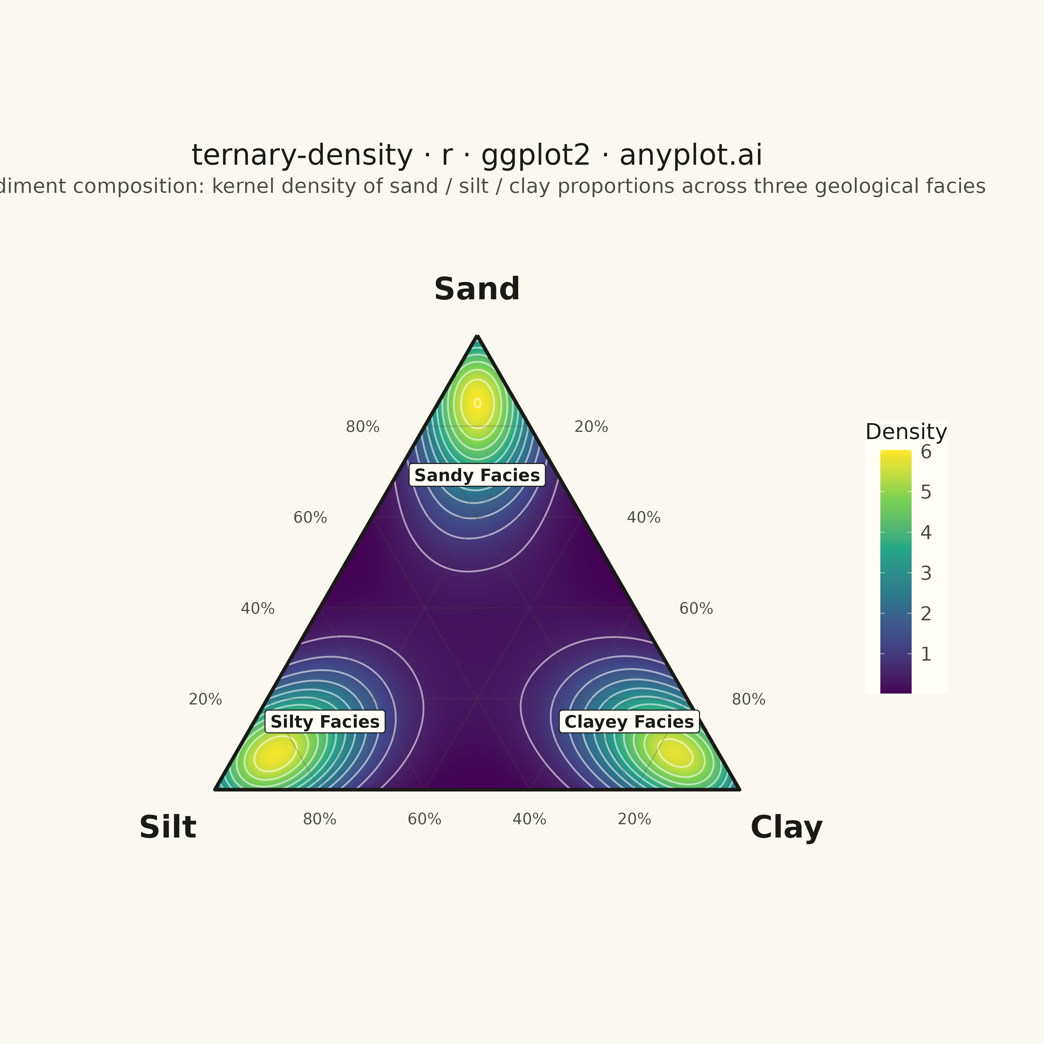
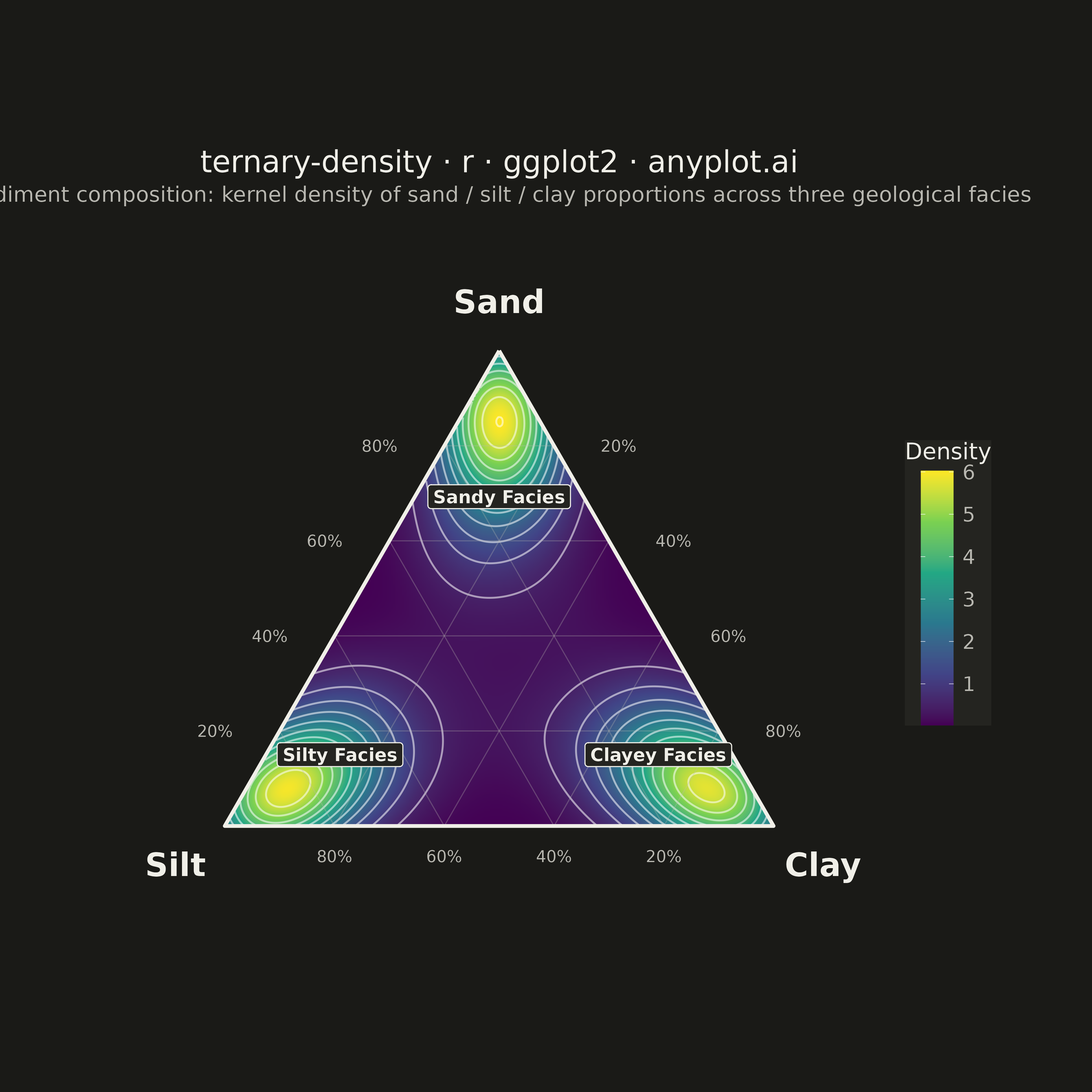
A ternary density plot combines a three-component ternary diagram with kernel density estimation to visualize where compositional data concentrates. Instead of showing individual points, this visualization uses a heatmap overlay to reveal the underlying probability distribution of compositions, making it ideal for identifying clusters, modes, and patterns in large compositional datasets.
#' anyplot.ai
#' ternary-density: Ternary Density Plot
#' Library: ggplot2 3.5.1 | R 4.4.1
#' Quality: 87/100 | Created: 2026-05-19

library(ggplot2)
library(MASS)
library(ragg)

set.seed(42)

# Theme tokens
THEME       <- Sys.getenv("ANYPLOT_THEME", "light")
PAGE_BG     <- if (THEME == "light") "#FAF8F1" else "#1A1A17"
ELEVATED_BG <- if (THEME == "light") "#FFFDF6" else "#242420"
INK         <- if (THEME == "light") "#1A1A17" else "#F0EFE8"
INK_SOFT    <- if (THEME == "light") "#4A4A44" else "#B8B7B0"

# Equilateral triangle height (side = 1)
TRI_H <- sqrt(3) / 2

# Data: sediment composition (sand / silt / clay) – three geological facies
n <- 600

# Sandy facies: concentrated near sand (top) vertex
sand1  <- rbeta(n, 8, 2)
split1 <- runif(n, 0.25, 0.75)
silt1  <- (1 - sand1) * split1
clay1  <- (1 - sand1) * (1 - split1)

# Silty facies: concentrated near silt (bottom-left) vertex
silt2  <- rbeta(n, 8, 2)
split2 <- runif(n, 0.25, 0.75)
sand2  <- (1 - silt2) * split2
clay2  <- (1 - silt2) * (1 - split2)

# Clayey facies: concentrated near clay (bottom-right) vertex
clay3  <- rbeta(n, 8, 2)
split3 <- runif(n, 0.25, 0.75)
sand3  <- (1 - clay3) * split3
silt3  <- (1 - clay3) * (1 - split3)

sand <- c(sand1, sand2, sand3)
silt <- c(silt1, silt2, silt3)
clay <- c(clay1, clay2, clay3)

# Ternary -> Cartesian: Sand=top (0.5, TRI_H), Silt=bottom-left (0,0), Clay=bottom-right (1,0)
cart_x <- 0.5 * sand + clay
cart_y <- TRI_H * sand

# KDE on Cartesian coordinates (triangle lies in [0,1] x [0, TRI_H])
n_grid  <- 300
kde     <- kde2d(cart_x, cart_y, n = n_grid, lims = c(0, 1, 0, TRI_H))

density_df   <- expand.grid(x = kde$x, y = kde$y)
density_df$z <- as.vector(kde$z)

# Mask density values outside the equilateral triangle
inside <- with(density_df,
  y >= 0 &
  x >= y / sqrt(3) &
  x <= 1 - y / sqrt(3)
)
density_df$z[!inside] <- NA

# Ternary reference grid at 20 / 40 / 60 / 80 % levels (three families of parallels)
grid_segs <- do.call(rbind, lapply(c(0.2, 0.4, 0.6, 0.8), function(f) {
  # Parallel to bottom (constant sand = f)
  yv <- f * TRI_H
  # Parallel to left edge (constant clay = f)
  # Parallel to right edge (constant silt = f)
  rbind(
    data.frame(x  = yv / sqrt(3),  xend = 1 - yv / sqrt(3), y  = yv,         yend = yv),
    data.frame(x  = f,             xend = 0.5*(1-f)+f,       y  = 0,          yend = (1-f)*TRI_H),
    data.frame(x  = 1-f,           xend = 0.5*(1-f),         y  = 0,          yend = (1-f)*TRI_H)
  )
}))

# Triangle border
tri_border <- data.frame(
  x = c(0.5, 0, 1, 0.5),
  y = c(TRI_H, 0, 0, TRI_H)
)

# Plot
p <- ggplot() +
  geom_raster(
    data = density_df,
    aes(x = x, y = y, fill = z),
    interpolate = TRUE
  ) +
  geom_contour(
    data      = density_df,
    aes(x = x, y = y, z = z),
    color     = "white",
    alpha     = 0.55,
    linewidth = 0.7,
    na.rm     = TRUE
  ) +
  geom_segment(
    data      = grid_segs,
    aes(x = x, xend = xend, y = y, yend = yend),
    color     = INK_SOFT,
    alpha     = 0.30,
    linewidth = 0.4
  ) +
  geom_path(
    data      = tri_border,
    aes(x = x, y = y),
    color     = INK,
    linewidth = 1.4
  ) +
  # Vertex labels
  annotate("text", x = 0.5,   y = TRI_H + 0.09, label = "Sand",
           color = INK, size = 9, fontface = "bold") +
  annotate("text", x = -0.09, y = -0.07,         label = "Silt",
           color = INK, size = 9, fontface = "bold") +
  annotate("text", x = 1.09,  y = -0.07,         label = "Clay",
           color = INK, size = 9, fontface = "bold") +
  scale_fill_viridis_c(
    option = "viridis",
    name   = "Density",
    na.value = "transparent",
    guide  = guide_colorbar(barwidth = 1.8, barheight = 14,
                            title.position = "top", title.hjust = 0.5)
  ) +
  coord_fixed(
    xlim = c(-0.16, 1.16),
    ylim = c(-0.16, TRI_H + 0.18)
  ) +
  labs(
    title    = "ternary-density · r · ggplot2 · anyplot.ai",
    subtitle = "Sediment composition: kernel density of sand / silt / clay proportions across three geological facies"
  ) +
  theme_void(base_size = 14) +
  theme(
    plot.background   = element_rect(fill = PAGE_BG, color = PAGE_BG),
    panel.background  = element_rect(fill = PAGE_BG, color = NA),
    plot.title        = element_text(color = INK,      size = 24, hjust = 0.5,
                                     margin = margin(t = 14, b = 6)),
    plot.subtitle     = element_text(color = INK_SOFT, size = 15, hjust = 0.5,
                                     margin = margin(b = 10)),
    legend.title      = element_text(color = INK,      size = 18),
    legend.text       = element_text(color = INK_SOFT, size = 14),
    legend.background = element_rect(fill = ELEVATED_BG, color = NA),
    legend.position   = "right",
    plot.margin       = margin(10, 80, 20, 80)
  )

# Save
ggsave(
  filename = sprintf("plot-%s.png", THEME),
  plot     = p,
  device   = ragg::agg_png,
  width    = 12,
  height   = 12,
  units    = "in",
  dpi      = 300
)
Runnable source as JSON, for any HTTP client: https://api.anyplot.ai/specs/ternary-density/ggplot2/code. Any spec id and library id listed in llms-full.txt fit the same URL shape; every URL below is complete and callable.
{
  "spec_id": "ternary-density",
  "language": "r",
  "library": "ggplot2",
  "page": "https://anyplot.ai/ternary-density/r/ggplot2",
  "hub": "https://anyplot.ai/ternary-density",
  "code_json": "https://api.anyplot.ai/specs/ternary-density/ggplot2/code",
  "spec_json": "https://api.anyplot.ai/specs/ternary-density",
  "render_light_png": "https://storage.googleapis.com/anyplot-images/plots/ternary-density/r/ggplot2/plot-light.png",
  "render_dark_png": "https://storage.googleapis.com/anyplot-images/plots/ternary-density/r/ggplot2/plot-dark.png",
  "quality_score": 87.0,
  "license": "MIT",
  "guide": "https://anyplot.ai/llms.txt"
}
Part of Ternary Density Plot on anyplot.ai.