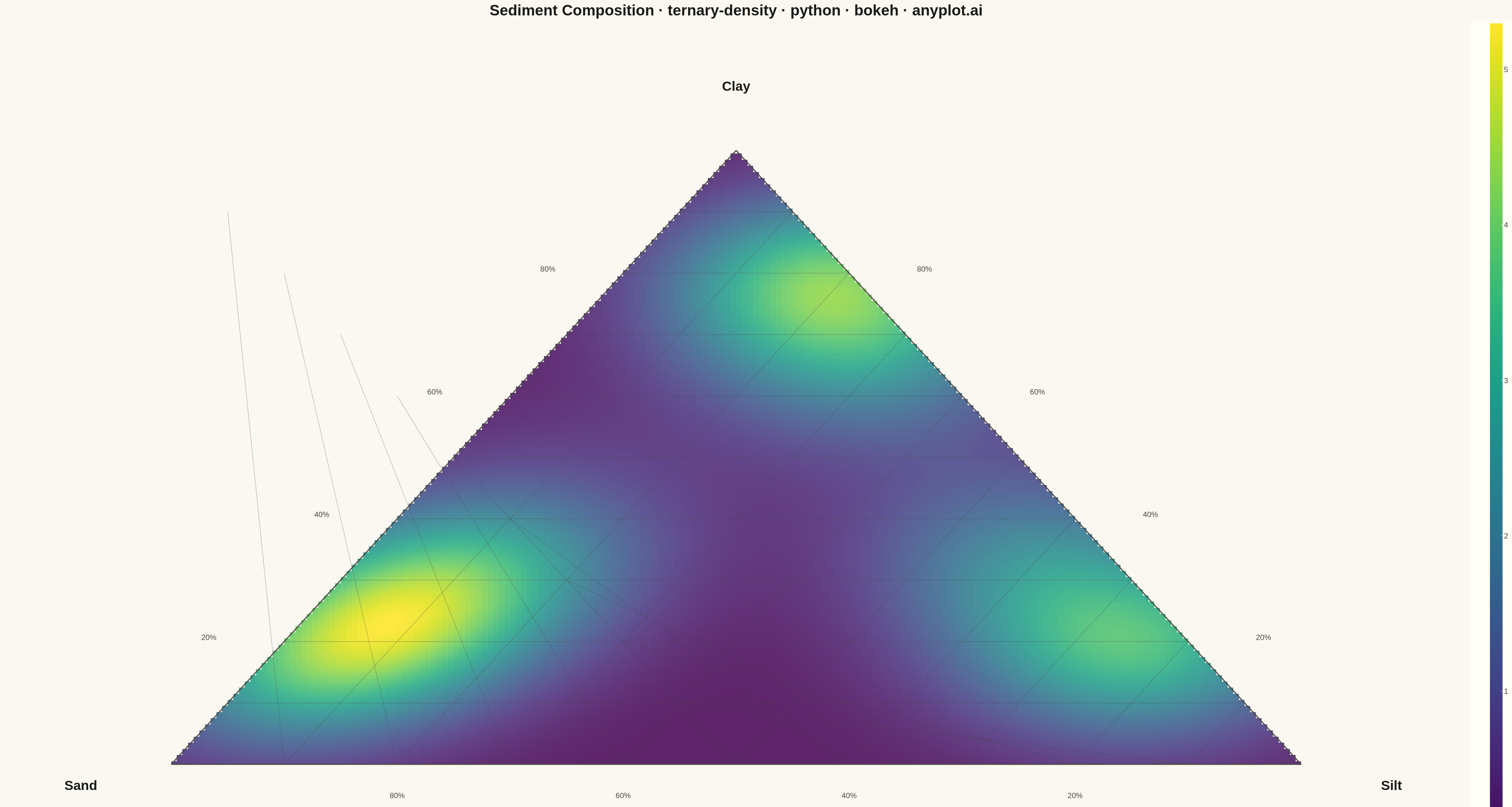
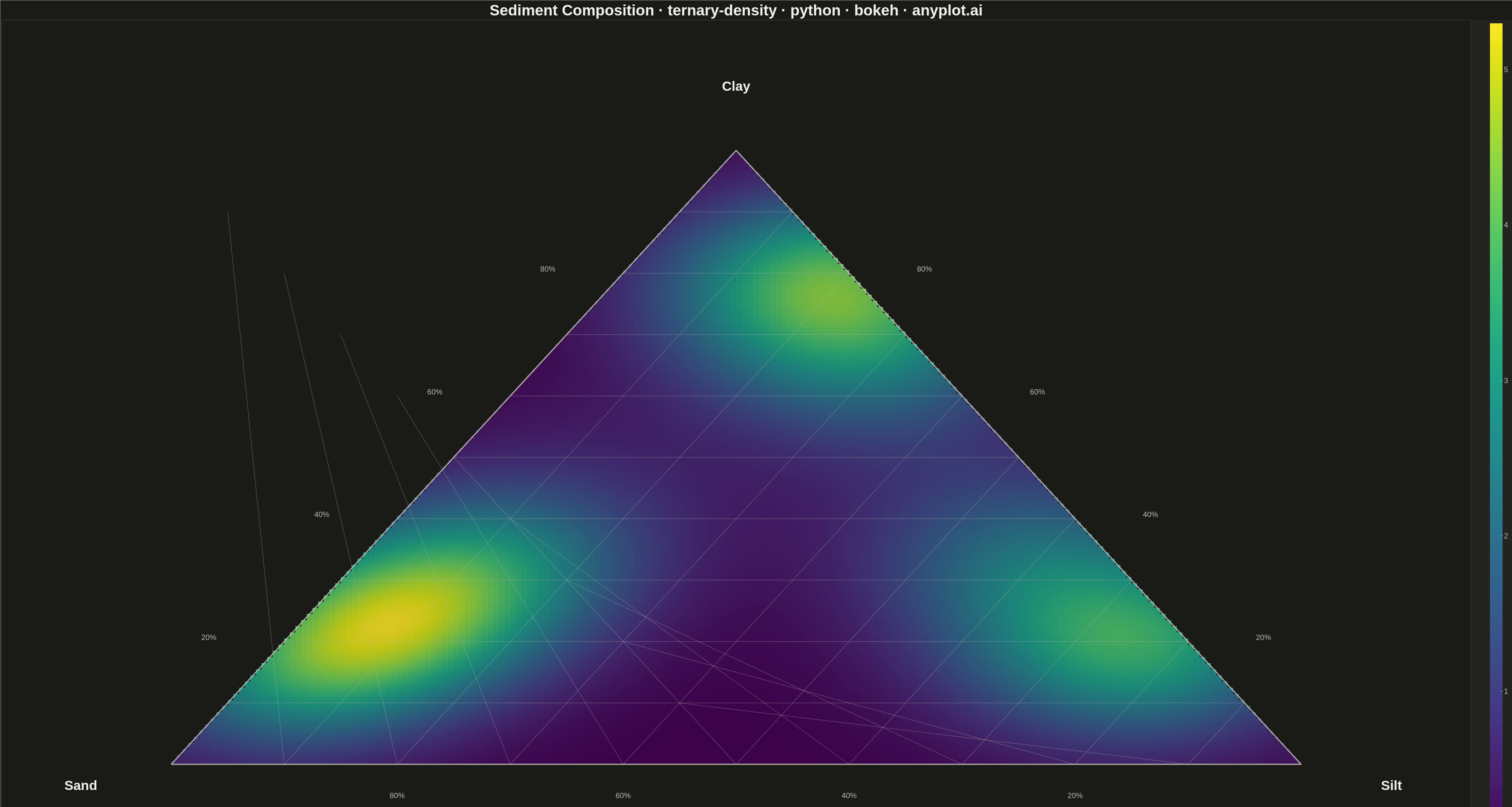
A ternary density plot combines a three-component ternary diagram with kernel density estimation to visualize where compositional data concentrates. Instead of showing individual points, this visualization uses a heatmap overlay to reveal the underlying probability distribution of compositions, making it ideal for identifying clusters, modes, and patterns in large compositional datasets.
""" anyplot.ai
ternary-density: Ternary Density Plot
Library: bokeh 3.9.0 | Python 3.13.13
Quality: 72/100 | Updated: 2026-05-19
"""

import numpy as np
from bokeh.io import export_png
from bokeh.models import ColorBar, Label, LinearColorMapper
from bokeh.plotting import figure
from scipy.stats import gaussian_kde


# Generate synthetic compositional data (sediment: sand/silt/clay)
np.random.seed(42)
n_points = 500

# Create three clusters of compositions
# Cluster 1: Sandy sediments (high sand)
n1 = 200
sand1 = np.random.beta(5, 2, n1) * 80 + 10
silt1 = np.random.beta(2, 3, n1) * (100 - sand1) * 0.6
clay1 = 100 - sand1 - silt1

# Cluster 2: Silty sediments (high silt)
n2 = 150
silt2 = np.random.beta(5, 2, n2) * 70 + 20
sand2 = np.random.beta(2, 3, n2) * (100 - silt2) * 0.5
clay2 = 100 - sand2 - silt2

# Cluster 3: Clayey sediments (high clay)
n3 = 150
clay3 = np.random.beta(5, 2, n3) * 60 + 30
sand3 = np.random.beta(2, 3, n3) * (100 - clay3) * 0.4
silt3 = 100 - sand3 - clay3

# Combine all clusters
sand = np.concatenate([sand1, sand2, sand3])
silt = np.concatenate([silt1, silt2, silt3])
clay = np.concatenate([clay1, clay2, clay3])

# Normalize to ensure they sum to 100
total = sand + silt + clay
sand = sand / total * 100
silt = silt / total * 100
clay = clay / total * 100


# Convert ternary to Cartesian coordinates
def ternary_to_cartesian(a, b, c):
    """Convert ternary coordinates (a, b, c) to Cartesian (x, y)."""
    total = a + b + c
    a, b, c = a / total, b / total, c / total
    x = 0.5 * (2 * b + c)
    y = (np.sqrt(3) / 2) * c
    return x, y


# Transform data points
x_data, y_data = ternary_to_cartesian(sand, silt, clay)

# Create density grid
grid_resolution = 200
x_grid = np.linspace(0, 1, grid_resolution)
y_grid = np.linspace(0, np.sqrt(3) / 2, grid_resolution)
xx, yy = np.meshgrid(x_grid, y_grid)

# Create mask for valid ternary region (inside the triangle)
# Triangle vertices: (0, 0), (1, 0), (0.5, sqrt(3)/2)
mask = np.zeros_like(xx, dtype=bool)
for i in range(grid_resolution):
    for j in range(grid_resolution):
        px, py = xx[i, j], yy[i, j]
        # Check if point is inside triangle using barycentric coordinates
        # Left edge: y <= sqrt(3) * x
        # Right edge: y <= sqrt(3) * (1 - x)
        # Bottom edge: y >= 0
        if py >= 0 and py <= np.sqrt(3) * px + 1e-6 and py <= np.sqrt(3) * (1 - px) + 1e-6:
            mask[i, j] = True

# Compute kernel density estimation
points = np.vstack([x_data, y_data])
kde = gaussian_kde(points, bw_method="scott")

# Evaluate on grid
positions = np.vstack([xx.ravel(), yy.ravel()])
density = kde(positions).reshape(xx.shape)

# Apply mask (set values outside triangle to NaN)
density_masked = np.where(mask, density, np.nan)

# Create figure (4800 x 2700 for landscape format)
p = figure(
    width=4800,
    height=2700,
    title="Sediment Composition · ternary-density · bokeh · pyplots.ai",
    x_range=(-0.15, 1.15),
    y_range=(-0.12, 1.05),
    tools="",
    toolbar_location=None,
)

# Remove axes and grid (we'll draw our own ternary grid)
p.xaxis.visible = False
p.yaxis.visible = False
p.xgrid.visible = False
p.ygrid.visible = False
p.outline_line_color = None

# Color mapper for density
color_mapper = LinearColorMapper(
    palette="Viridis256", low=np.nanmin(density_masked), high=np.nanmax(density_masked), nan_color="rgba(0, 0, 0, 0)"
)

# Plot density as image
p.image(image=[density_masked], x=0, y=0, dw=1, dh=np.sqrt(3) / 2, color_mapper=color_mapper, alpha=0.85)

# Triangle vertices
tri_x = [0, 1, 0.5, 0]
tri_y = [0, 0, np.sqrt(3) / 2, 0]

# Draw triangle outline
p.line(tri_x, tri_y, line_width=4, line_color="#306998", line_alpha=0.9)

# Draw grid lines inside triangle
grid_alpha = 0.4
grid_width = 2
grid_color = "#306998"

# Draw lines parallel to each edge (10%, 20%, ..., 90%)
for pct in [0.1, 0.2, 0.3, 0.4, 0.5, 0.6, 0.7, 0.8, 0.9]:
    # Lines parallel to bottom edge (constant clay %)
    y_line = pct * np.sqrt(3) / 2
    x_left = pct / 2
    x_right = 1 - pct / 2
    p.line([x_left, x_right], [y_line, y_line], line_width=grid_width, line_color=grid_color, line_alpha=grid_alpha)

    # Lines parallel to left edge (constant silt %)
    x_start = pct
    y_start = 0
    x_end = pct / 2 + 0.5
    y_end = (1 - pct) * np.sqrt(3) / 2
    p.line([x_start, x_end], [y_start, y_end], line_width=grid_width, line_color=grid_color, line_alpha=grid_alpha)

    # Lines parallel to right edge (constant sand %)
    x_start = 1 - pct
    y_start = 0
    x_end = (1 - pct) / 2
    y_end = pct * np.sqrt(3) / 2
    p.line([x_start, x_end], [y_start, y_end], line_width=grid_width, line_color=grid_color, line_alpha=grid_alpha)

# Add vertex labels
label_font_size = "32pt"
label_offset = 0.08

# Sand (bottom left)
sand_label = Label(
    x=0 - label_offset,
    y=0 - label_offset / 2,
    text="Sand",
    text_font_size=label_font_size,
    text_color="#306998",
    text_font_style="bold",
    text_align="center",
)
p.add_layout(sand_label)

# Silt (bottom right)
silt_label = Label(
    x=1 + label_offset,
    y=0 - label_offset / 2,
    text="Silt",
    text_font_size=label_font_size,
    text_color="#306998",
    text_font_style="bold",
    text_align="center",
)
p.add_layout(silt_label)

# Clay (top)
clay_label = Label(
    x=0.5,
    y=np.sqrt(3) / 2 + label_offset,
    text="Clay",
    text_font_size=label_font_size,
    text_color="#306998",
    text_font_style="bold",
    text_align="center",
)
p.add_layout(clay_label)

# Add percentage labels along edges
tick_font_size = "18pt"

# Bottom edge (Sand percentage, from left to right is 100% to 0%)
for pct in [20, 40, 60, 80]:
    x_pos = pct / 100
    p.add_layout(
        Label(
            x=x_pos,
            y=-0.05,
            text=f"{100 - pct}%",
            text_font_size=tick_font_size,
            text_color="#666666",
            text_align="center",
        )
    )

# Left edge (Clay percentage, from bottom to top is 0% to 100%)
for pct in [20, 40, 60, 80]:
    x_pos = pct / 100 / 2
    y_pos = pct / 100 * np.sqrt(3) / 2
    p.add_layout(
        Label(
            x=x_pos - 0.06,
            y=y_pos,
            text=f"{pct}%",
            text_font_size=tick_font_size,
            text_color="#666666",
            text_align="right",
        )
    )

# Right edge (Silt percentage)
for pct in [20, 40, 60, 80]:
    x_pos = 1 - pct / 100 / 2
    y_pos = pct / 100 * np.sqrt(3) / 2
    p.add_layout(
        Label(
            x=x_pos + 0.06,
            y=y_pos,
            text=f"{pct}%",
            text_font_size=tick_font_size,
            text_color="#666666",
            text_align="left",
        )
    )

# Add color bar
color_bar = ColorBar(
    color_mapper=color_mapper,
    width=40,
    location=(0, 0),
    title="Density",
    title_text_font_size="24pt",
    major_label_text_font_size="18pt",
    title_text_color="#306998",
    major_label_text_color="#666666",
    title_standoff=15,
    margin=20,
)
p.add_layout(color_bar, "right")

# Title styling
p.title.text_font_size = "36pt"
p.title.text_color = "#306998"
p.title.align = "center"

# Save
export_png(p, filename="plot.png")
Runnable source as JSON, for any HTTP client: https://api.anyplot.ai/specs/ternary-density/bokeh/code. Any spec id and library id listed in llms-full.txt fit the same URL shape; every URL below is complete and callable.
{
  "spec_id": "ternary-density",
  "language": "python",
  "library": "bokeh",
  "page": "https://anyplot.ai/ternary-density/python/bokeh",
  "hub": "https://anyplot.ai/ternary-density",
  "code_json": "https://api.anyplot.ai/specs/ternary-density/bokeh/code",
  "spec_json": "https://api.anyplot.ai/specs/ternary-density",
  "render_light_png": "https://storage.googleapis.com/anyplot-images/plots/ternary-density/python/bokeh/plot-light.png",
  "render_dark_png": "https://storage.googleapis.com/anyplot-images/plots/ternary-density/python/bokeh/plot-dark.png",
  "interactive_light_html": "https://storage.googleapis.com/anyplot-images/plots/ternary-density/python/bokeh/plot-light.html",
  "interactive_dark_html": "https://storage.googleapis.com/anyplot-images/plots/ternary-density/python/bokeh/plot-dark.html",
  "quality_score": 72.0,
  "license": "MIT",
  "guide": "https://anyplot.ai/llms.txt"
}
Part of Ternary Density Plot on anyplot.ai.