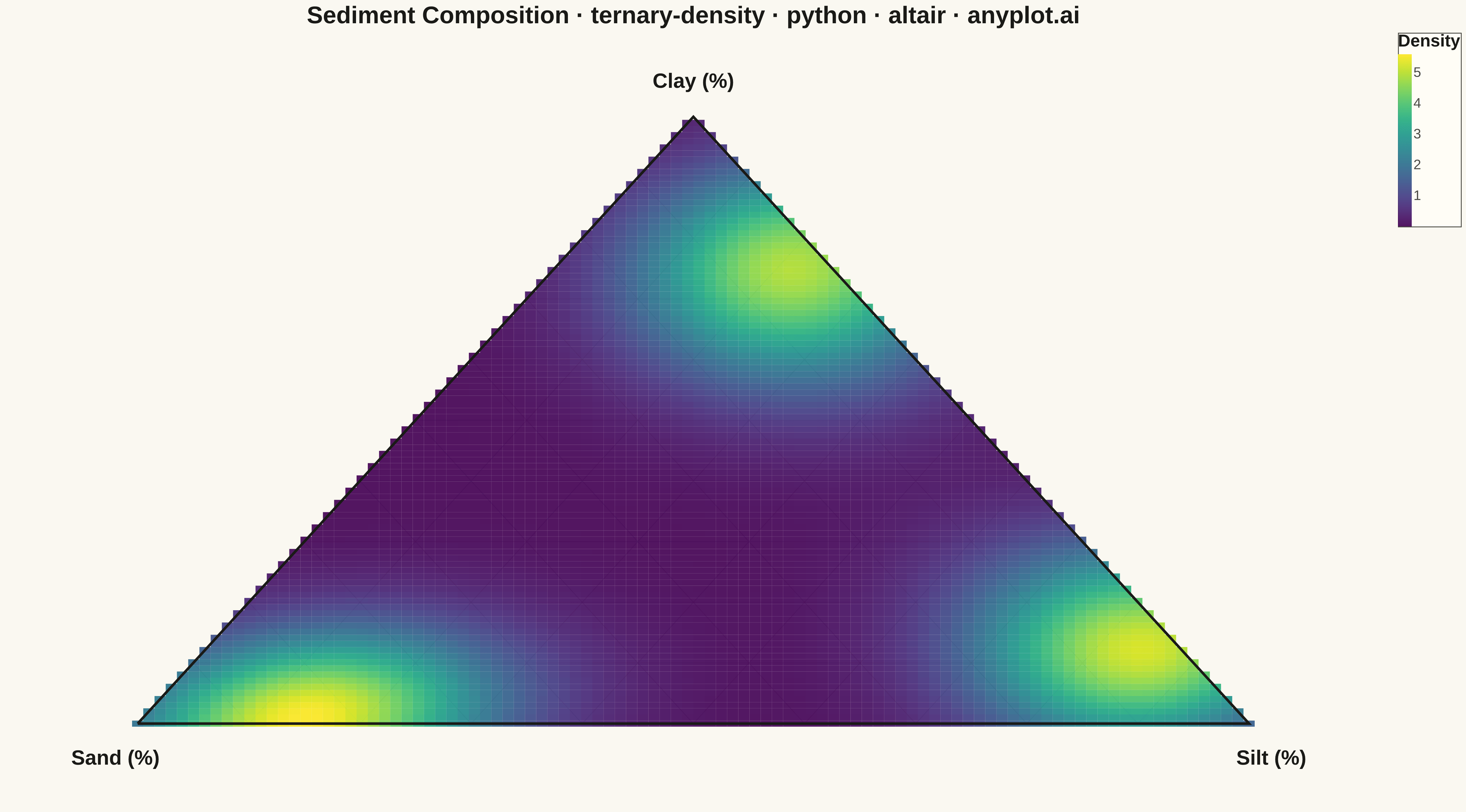
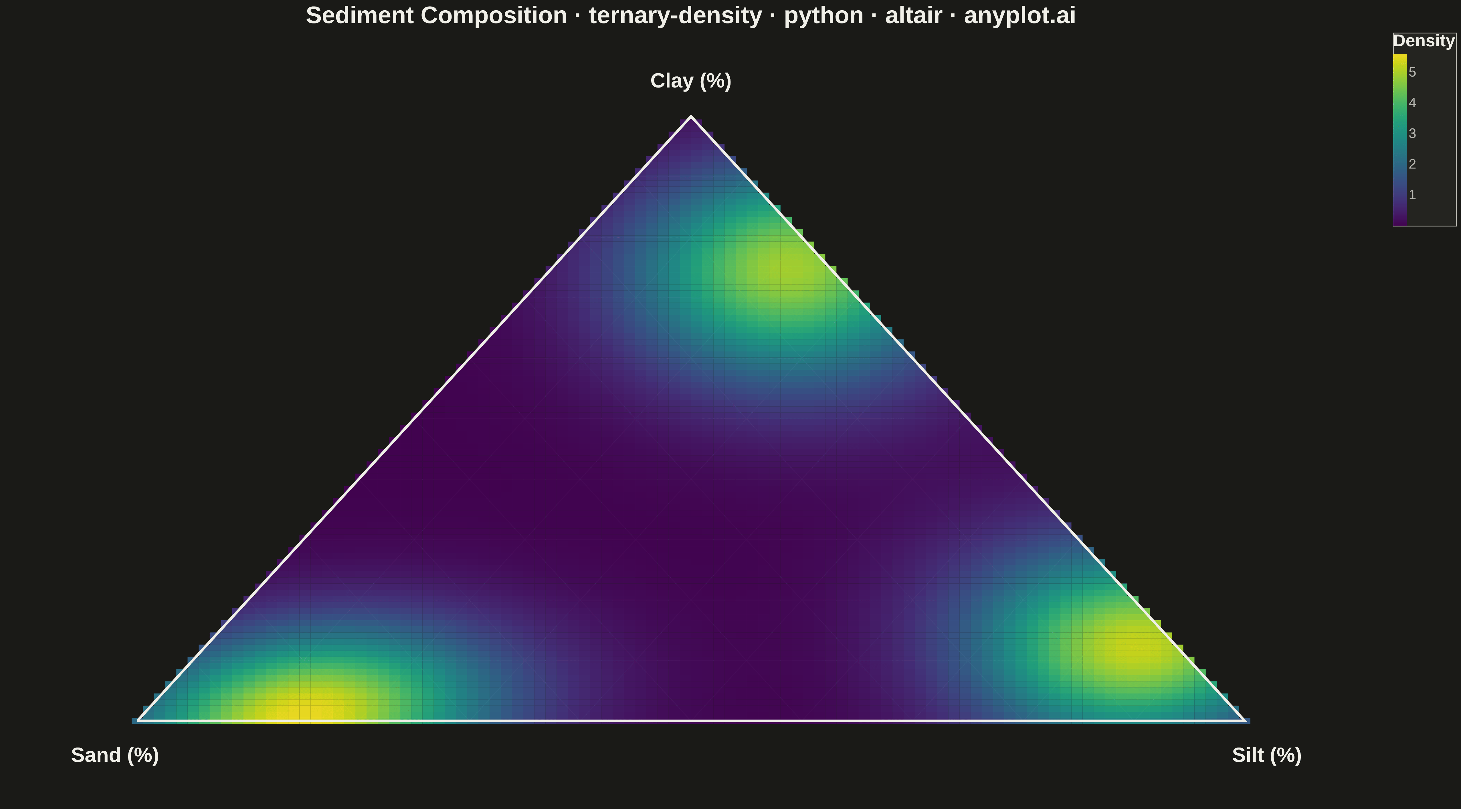
A ternary density plot combines a three-component ternary diagram with kernel density estimation to visualize where compositional data concentrates. Instead of showing individual points, this visualization uses a heatmap overlay to reveal the underlying probability distribution of compositions, making it ideal for identifying clusters, modes, and patterns in large compositional datasets.
""" anyplot.ai
ternary-density: Ternary Density Plot
Library: altair 6.1.0 | Python 3.13.13
Quality: 90/100 | Updated: 2026-05-19
"""

import os

import altair as alt
import numpy as np
import pandas as pd
from scipy.stats import gaussian_kde


# Theme tokens
THEME = os.getenv("ANYPLOT_THEME", "light")
PAGE_BG = "#FAF8F1" if THEME == "light" else "#1A1A17"
ELEVATED_BG = "#FFFDF6" if THEME == "light" else "#242420"
INK = "#1A1A17" if THEME == "light" else "#F0EFE8"
INK_SOFT = "#4A4A44" if THEME == "light" else "#B8B7B0"

# Data — clustered sediment compositions (sand/silt/clay)
np.random.seed(42)
n_per_cluster = 400

# Cluster 1: Sandy sediment (high sand, low clay)
c1_sand = np.random.beta(12, 2, n_per_cluster) * 80 + 15
c1_clay = np.random.beta(2, 8, n_per_cluster) * (100 - c1_sand) * 0.3
c1_silt = 100 - c1_sand - c1_clay

# Cluster 2: Silty sediment (high silt)
c2_silt = np.random.beta(10, 2, n_per_cluster) * 70 + 25
c2_sand = np.random.beta(3, 6, n_per_cluster) * (100 - c2_silt) * 0.7
c2_clay = 100 - c2_silt - c2_sand

# Cluster 3: Clay-rich sediment (high clay)
c3_clay = np.random.beta(8, 3, n_per_cluster) * 60 + 30
c3_sand = np.random.beta(2, 5, n_per_cluster) * (100 - c3_clay) * 0.5
c3_silt = 100 - c3_clay - c3_sand

# Combine and normalize to exact 100%
sand = np.concatenate([c1_sand, c2_sand, c3_sand])
silt = np.concatenate([c1_silt, c2_silt, c3_silt])
clay = np.concatenate([c1_clay, c2_clay, c3_clay])
sand = np.clip(sand, 0.1, 99.8)
silt = np.clip(silt, 0.1, 99.8)
clay = np.clip(clay, 0.1, 99.8)
total = sand + silt + clay
sand, silt, clay = sand / total * 100, silt / total * 100, clay / total * 100

# Ternary → Cartesian: Sand=(0,0), Silt=(1,0), Clay=(0.5, √3/2)
sqrt3_2 = np.sqrt(3) / 2
x_pts = 0.5 * (2 * silt + clay) / 100
y_pts = sqrt3_2 * clay / 100

# KDE on the transformed coordinates
grid_res = 100
x_grid = np.linspace(0, 1, grid_res)
y_grid = np.linspace(0, sqrt3_2, grid_res)
xx, yy = np.meshgrid(x_grid, y_grid)
kde = gaussian_kde(np.vstack([x_pts, y_pts]), bw_method="scott")
density = kde(np.vstack([xx.ravel(), yy.ravel()])).reshape(xx.shape)

# Triangle mask (half-plane method)
margin = 0.005
inside = (yy >= -margin) & (np.sqrt(3) * xx + yy <= np.sqrt(3) + margin) & (yy - np.sqrt(3) * xx <= margin)

# Cell half-widths for mark_rect (pixel-perfect coverage)
dx = (x_grid[1] - x_grid[0]) / 2
dy = (y_grid[1] - y_grid[0]) / 2

# Density DataFrame — explicit cell bounds for clean edges
density_rows = [
    {"x1": xx[i, j] - dx, "x2": xx[i, j] + dx, "y1": yy[i, j] - dy, "y2": yy[i, j] + dy, "density": density[i, j]}
    for i in range(grid_res)
    for j in range(grid_res)
    if inside[i, j]
]
density_df = pd.DataFrame(density_rows)

# Triangle outline vertices
triangle_df = pd.DataFrame({"x": [0, 1, 0.5, 0], "y": [0, 0, sqrt3_2, 0], "order": [0, 1, 2, 3]})

# Ternary grid lines (10% intervals for all three axes)
grid_lines = []
for i in range(1, 10):
    frac = i / 10
    # Constant clay (horizontal)
    y_val = frac * sqrt3_2
    x_left = y_val / np.sqrt(3)
    x_right = 1 - y_val / np.sqrt(3)
    grid_lines += [
        {"x": x_left, "y": y_val, "line": f"h{i}", "o": 0},
        {"x": x_right, "y": y_val, "line": f"h{i}", "o": 1},
    ]
    # Constant sand
    grid_lines += [
        {"x": frac, "y": 0, "line": f"s{i}", "o": 0},
        {"x": frac / 2, "y": frac * sqrt3_2, "line": f"s{i}", "o": 1},
    ]
    # Constant silt
    grid_lines += [
        {"x": 1 - frac, "y": 0, "line": f"t{i}", "o": 0},
        {"x": 1 - frac / 2, "y": frac * sqrt3_2, "line": f"t{i}", "o": 1},
    ]
grid_df = pd.DataFrame(grid_lines)

# Vertex labels
labels_df = pd.DataFrame(
    {"x": [-0.02, 1.02, 0.5], "y": [-0.05, -0.05, sqrt3_2 + 0.05], "label": ["Sand (%)", "Silt (%)", "Clay (%)"]}
)

# Shared scale domains for all layers
X_DOMAIN = [-0.12, 1.12]
Y_DOMAIN = [-0.12, sqrt3_2 + 0.12]

# Density heatmap — mark_rect with explicit cell bounds
heatmap = (
    alt.Chart(density_df)
    .mark_rect(opacity=0.92)
    .encode(
        x=alt.X("x1:Q", scale=alt.Scale(domain=X_DOMAIN), axis=None),
        x2=alt.X2("x2:Q"),
        y=alt.Y("y1:Q", scale=alt.Scale(domain=Y_DOMAIN), axis=None),
        y2=alt.Y2("y2:Q"),
        color=alt.Color(
            "density:Q",
            scale=alt.Scale(scheme="viridis"),
            legend=alt.Legend(title="Density", titleFontSize=20, labelFontSize=16, orient="right"),
        ),
    )
)

# Triangle outline
triangle = (
    alt.Chart(triangle_df)
    .mark_line(color=INK, strokeWidth=3)
    .encode(
        x=alt.X("x:Q", scale=alt.Scale(domain=X_DOMAIN), axis=None),
        y=alt.Y("y:Q", scale=alt.Scale(domain=Y_DOMAIN), axis=None),
        order="order:O",
    )
)

# Grid lines
grid = (
    alt.Chart(grid_df)
    .mark_line(color=INK_SOFT, strokeWidth=1, opacity=0.35)
    .encode(
        x=alt.X("x:Q", scale=alt.Scale(domain=X_DOMAIN), axis=None),
        y=alt.Y("y:Q", scale=alt.Scale(domain=Y_DOMAIN), axis=None),
        detail="line:N",
        order="o:O",
    )
)

# Vertex labels
labels = (
    alt.Chart(labels_df)
    .mark_text(fontSize=24, fontWeight="bold", color=INK)
    .encode(
        x=alt.X("x:Q", scale=alt.Scale(domain=X_DOMAIN), axis=None),
        y=alt.Y("y:Q", scale=alt.Scale(domain=Y_DOMAIN), axis=None),
        text="label:N",
    )
)

# Compose layers
chart = (
    alt.layer(grid, heatmap, triangle, labels)
    .properties(
        background=PAGE_BG,
        width=1600,
        height=900,
        title=alt.Title(
            "Sediment Composition · ternary-density · python · altair · anyplot.ai", fontSize=28, color=INK
        ),
    )
    .configure_view(fill=PAGE_BG, strokeWidth=0)
    .configure_legend(fillColor=ELEVATED_BG, strokeColor=INK_SOFT, labelColor=INK_SOFT, titleColor=INK)
)

# Save
chart.save(f"plot-{THEME}.png", scale_factor=3.0)
chart.save(f"plot-{THEME}.html")
Runnable source as JSON, for any HTTP client: https://api.anyplot.ai/specs/ternary-density/altair/code. Any spec id and library id listed in llms-full.txt fit the same URL shape; every URL below is complete and callable.
{
  "spec_id": "ternary-density",
  "language": "python",
  "library": "altair",
  "page": "https://anyplot.ai/ternary-density/python/altair",
  "hub": "https://anyplot.ai/ternary-density",
  "code_json": "https://api.anyplot.ai/specs/ternary-density/altair/code",
  "spec_json": "https://api.anyplot.ai/specs/ternary-density",
  "render_light_png": "https://storage.googleapis.com/anyplot-images/plots/ternary-density/python/altair/plot-light.png",
  "render_dark_png": "https://storage.googleapis.com/anyplot-images/plots/ternary-density/python/altair/plot-dark.png",
  "interactive_light_html": "https://storage.googleapis.com/anyplot-images/plots/ternary-density/python/altair/plot-light.html",
  "interactive_dark_html": "https://storage.googleapis.com/anyplot-images/plots/ternary-density/python/altair/plot-dark.html",
  "quality_score": 90.0,
  "license": "MIT",
  "guide": "https://anyplot.ai/llms.txt"
}
Part of Ternary Density Plot on anyplot.ai.