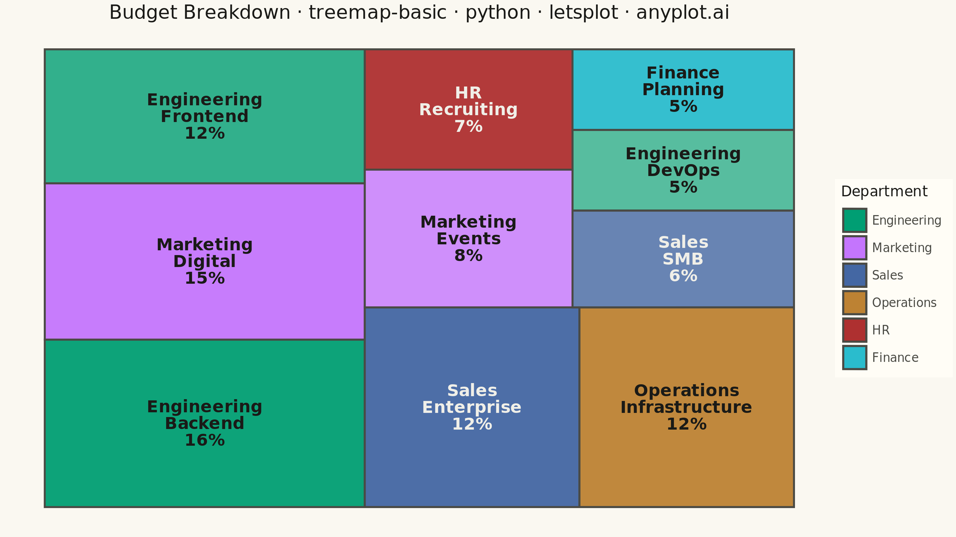
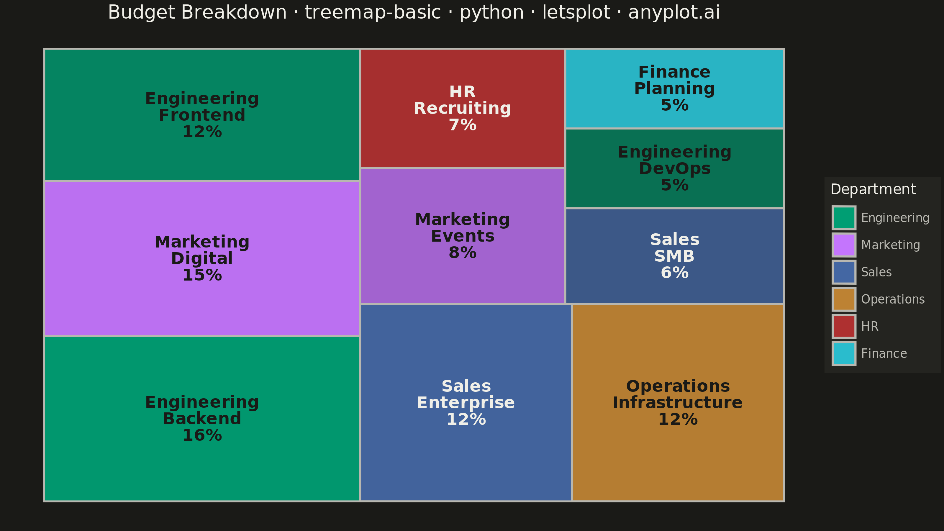
A treemap displaying hierarchical data as nested rectangles, where each rectangle's area is proportional to its value. This visualization excels at showing part-to-whole relationships in hierarchical structures, making it easy to spot large and small items at a glance. Treemaps efficiently use screen space to display large amounts of hierarchical data in a compact form.
""" anyplot.ai
treemap-basic: Basic Treemap
Library: letsplot 4.11.0 | Python 3.13.14
Quality: 88/100 | Updated: 2026-08-04
"""

import os

import pandas as pd
from lets_plot import (
    LetsPlot,
    aes,
    element_blank,
    element_rect,
    element_text,
    geom_rect,
    geom_text,
    ggplot,
    ggsize,
    labs,
    scale_alpha_identity,
    scale_color_identity,
    scale_fill_manual,
    theme,
    theme_void,
)
from lets_plot.export import ggsave


LetsPlot.setup_html()

# Theme tokens
THEME = os.getenv("ANYPLOT_THEME", "light")
PAGE_BG = "#FAF8F1" if THEME == "light" else "#1A1A17"
ELEVATED_BG = "#FFFDF6" if THEME == "light" else "#242420"
INK = "#1A1A17" if THEME == "light" else "#F0EFE8"
INK_SOFT = "#4A4A44" if THEME == "light" else "#B8B7B0"

# Okabe-Ito palette for consistent color mapping across categories
IMPRINT = ["#009E73", "#C475FD", "#4467A3", "#BD8233", "#AE3030", "#2ABCCD", "#954477"]

# Data - Budget allocation with two-level hierarchy
# Departments (main) and projects/teams (sub) for realistic budget breakdown
data = {
    "category": [
        "Engineering",
        "Engineering",
        "Engineering",
        "Marketing",
        "Marketing",
        "Sales",
        "Sales",
        "Operations",
        "HR",
        "Finance",
    ],
    "subcategory": [
        "Backend",
        "Frontend",
        "DevOps",
        "Digital",
        "Events",
        "Enterprise",
        "SMB",
        "Infrastructure",
        "Recruiting",
        "Planning",
    ],
    "value": [15, 12, 5, 14, 8, 12, 6, 12, 7, 5],
}

df_data = pd.DataFrame(data)
df_data = df_data.sort_values("value", ascending=False).reset_index(drop=True)


def squarify(values, x, y, width, height):
    """Compute treemap rectangles using squarify algorithm.

    Tracks a running remaining-total and remaining width/height (rather than
    the fixed global values) so consumed area always matches the actual
    remaining container, guaranteeing the tiling fully fills the bounding box.
    """
    if len(values) == 0:
        return []

    remaining_total = sum(values)
    if remaining_total == 0:
        return []

    rects = []
    remaining_values = list(values)
    remaining_x, remaining_y = x, y
    remaining_w, remaining_h = width, height

    while remaining_values:
        if remaining_w >= remaining_h:
            row_values = []
            row_sum = 0
            best_ratio = float("inf")

            for v in remaining_values:
                test_values = row_values + [v]
                test_sum = row_sum + v
                row_width = (test_sum / remaining_total) * remaining_w if remaining_total > 0 else 0

                if row_width > 0:
                    worst_ratio = 0
                    for rv in test_values:
                        rect_height = (rv / test_sum) * remaining_h if test_sum > 0 else 0
                        ratio = (
                            max(row_width / rect_height, rect_height / row_width) if rect_height > 0 else float("inf")
                        )
                        worst_ratio = max(worst_ratio, ratio)

                    if worst_ratio <= best_ratio:
                        best_ratio = worst_ratio
                        row_values = test_values
                        row_sum = test_sum
                    else:
                        break
                else:
                    row_values = test_values
                    row_sum = test_sum

            row_width = (row_sum / remaining_total) * remaining_w if remaining_total > 0 else 0
            current_y = remaining_y
            for rv in row_values:
                rect_height = (rv / row_sum) * remaining_h if row_sum > 0 else 0
                rects.append((remaining_x, current_y, row_width, rect_height))
                current_y += rect_height

            remaining_x += row_width
            remaining_w -= row_width
            remaining_total -= row_sum
            remaining_values = remaining_values[len(row_values) :]
        else:
            col_values = []
            col_sum = 0
            best_ratio = float("inf")

            for v in remaining_values:
                test_values = col_values + [v]
                test_sum = col_sum + v
                col_height = (test_sum / remaining_total) * remaining_h if remaining_total > 0 else 0

                if col_height > 0:
                    worst_ratio = 0
                    for cv in test_values:
                        rect_width = (cv / test_sum) * remaining_w if test_sum > 0 else 0
                        ratio = (
                            max(col_height / rect_width, rect_width / col_height) if rect_width > 0 else float("inf")
                        )
                        worst_ratio = max(worst_ratio, ratio)

                    if worst_ratio <= best_ratio:
                        best_ratio = worst_ratio
                        col_values = test_values
                        col_sum = test_sum
                    else:
                        break
                else:
                    col_values = test_values
                    col_sum = test_sum

            col_height = (col_sum / remaining_total) * remaining_h if remaining_total > 0 else 0
            current_x = remaining_x
            for cv in col_values:
                rect_width = (cv / col_sum) * remaining_w if col_sum > 0 else 0
                rects.append((current_x, remaining_y, rect_width, col_height))
                current_x += rect_width

            remaining_y += col_height
            remaining_h -= col_height
            remaining_total -= col_sum
            remaining_values = remaining_values[len(col_values) :]

    return rects


# Compute treemap layout
rects = squarify(df_data["value"].tolist(), 0, 0, 100, 100)

# Build rectangle dataframe
rect_df = pd.DataFrame(
    {
        "xmin": [r[0] for r in rects],
        "ymin": [r[1] for r in rects],
        "xmax": [r[0] + r[2] for r in rects],
        "ymax": [r[1] + r[3] for r in rects],
        "category": df_data["category"].tolist(),
        "subcategory": df_data["subcategory"].tolist(),
        "value": df_data["value"].tolist(),
    }
)

# Calculate label positions
rect_df["label_x"] = (rect_df["xmin"] + rect_df["xmax"]) / 2
rect_df["label_y"] = (rect_df["ymin"] + rect_df["ymax"]) / 2
rect_df["width"] = rect_df["xmax"] - rect_df["xmin"]
rect_df["height"] = rect_df["ymax"] - rect_df["ymin"]

# Shading intensity by nesting depth: within each department, the largest
# cost center is fully opaque and successive ones step down in alpha, giving
# a visual cue for the subcategory hierarchy beyond color alone.
rect_df["subcat_rank"] = rect_df.groupby("category")["value"].rank(ascending=False, method="first") - 1
rect_df["shade_alpha"] = (0.95 - 0.15 * rect_df["subcat_rank"]).clip(lower=0.55)

# Create adaptive labels for improved readability
total_value = df_data["value"].sum()


def make_label(row):
    w, h = row["width"], row["height"]
    pct = row["value"] / total_value * 100
    # Large rectangles: show both category and subcategory with percentage
    if w > 20 and h > 12:
        return f"{row['category']}\n{row['subcategory']}\n{pct:.0f}%"
    # Medium rectangles: subcategory and percentage
    elif w > 12 and h > 8:
        return f"{row['subcategory']}\n{pct:.0f}%"
    # Small rectangles: just subcategory
    elif w > 8 and h > 6:
        return f"{row['subcategory']}"
    # Very small: no label (visible in legend)
    return ""


rect_df["label"] = rect_df.apply(make_label, axis=1)

# Map categories to Okabe-Ito colors
unique_categories = df_data["category"].unique().tolist()
category_colors = {cat: IMPRINT[i % len(IMPRINT)] for i, cat in enumerate(unique_categories)}
color_values = [category_colors[cat] for cat in unique_categories]

# Per-swatch label color: pick whichever of near-black/near-white ink gives
# the higher WCAG contrast against that category's fill, so labels stay
# legible on both light swatches (e.g. lavender) and dark ones (e.g. red).
DARK_INK = "#1A1A17"
LIGHT_INK = "#F0EFE8"


def relative_luminance(hex_color):
    r, g, b = (int(hex_color.lstrip("#")[i : i + 2], 16) / 255 for i in (0, 2, 4))

    def channel(c):
        return c / 12.92 if c <= 0.03928 else ((c + 0.055) / 1.055) ** 2.4

    r, g, b = channel(r), channel(g), channel(b)
    return 0.2126 * r + 0.7152 * g + 0.0722 * b


def contrast_ratio(lum_a, lum_b):
    lighter, darker = max(lum_a, lum_b), min(lum_a, lum_b)
    return (lighter + 0.05) / (darker + 0.05)


def best_label_color(bg_hex):
    bg_lum = relative_luminance(bg_hex)
    dark_contrast = contrast_ratio(bg_lum, relative_luminance(DARK_INK))
    light_contrast = contrast_ratio(bg_lum, relative_luminance(LIGHT_INK))
    return DARK_INK if dark_contrast >= light_contrast else LIGHT_INK


label_colors = {cat: best_label_color(color) for cat, color in category_colors.items()}
rect_df["label_color"] = rect_df["category"].map(label_colors)
TEXT_SIZE = 7

# Create the plot
plot = (
    ggplot(rect_df)
    + geom_rect(
        aes(xmin="xmin", ymin="ymin", xmax="xmax", ymax="ymax", fill="category", alpha="shade_alpha"),
        color=INK_SOFT,
        size=0.7,
    )
    + geom_text(aes(x="label_x", y="label_y", label="label", color="label_color"), size=TEXT_SIZE, fontface="bold")
    + scale_fill_manual(values=color_values)
    + scale_color_identity()
    + scale_alpha_identity()
    + labs(title="Budget Breakdown · treemap-basic · python · letsplot · anyplot.ai", fill="Department")
    + theme_void()
    + theme(
        plot_background=element_rect(fill=PAGE_BG, color=PAGE_BG),
        plot_title=element_text(size=16, color=INK, hjust=0.5),
        legend_title=element_text(size=12, color=INK),
        legend_text=element_text(size=10, color=INK_SOFT),
        legend_background=element_rect(fill=ELEVATED_BG, color=INK_SOFT),
        legend_position="right",
        axis_title=element_blank(),
        axis_text=element_blank(),
    )
    + ggsize(800, 450)
)

# Save outputs with theme suffix
ggsave(plot, f"plot-{THEME}.png", path=".", scale=4)
ggsave(plot, f"plot-{THEME}.html", path=".")
Runnable source as JSON, for any HTTP client: https://api.anyplot.ai/specs/treemap-basic/letsplot/code. Any spec id and library id listed in llms-full.txt fit the same URL shape; every URL below is complete and callable.
{
  "spec_id": "treemap-basic",
  "language": "python",
  "library": "letsplot",
  "page": "https://anyplot.ai/treemap-basic/python/letsplot",
  "hub": "https://anyplot.ai/treemap-basic",
  "code_json": "https://api.anyplot.ai/specs/treemap-basic/letsplot/code",
  "spec_json": "https://api.anyplot.ai/specs/treemap-basic",
  "render_light_png": "https://storage.googleapis.com/anyplot-images/plots/treemap-basic/python/letsplot/plot-light.png",
  "render_dark_png": "https://storage.googleapis.com/anyplot-images/plots/treemap-basic/python/letsplot/plot-dark.png",
  "interactive_light_html": "https://storage.googleapis.com/anyplot-images/plots/treemap-basic/python/letsplot/plot-light.html",
  "interactive_dark_html": "https://storage.googleapis.com/anyplot-images/plots/treemap-basic/python/letsplot/plot-dark.html",
  "quality_score": 88.0,
  "license": "MIT",
  "guide": "https://anyplot.ai/llms.txt"
}
Part of Basic Treemap on anyplot.ai.