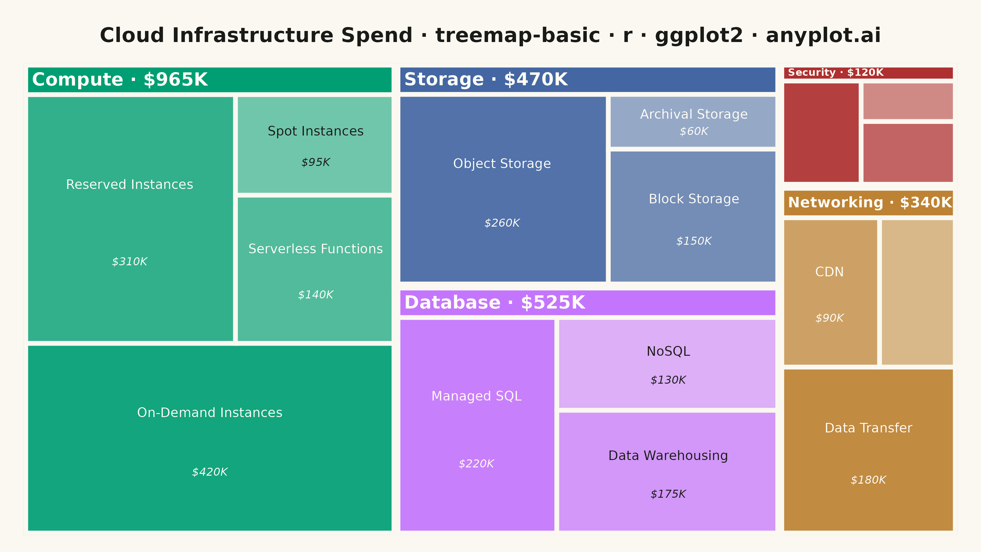
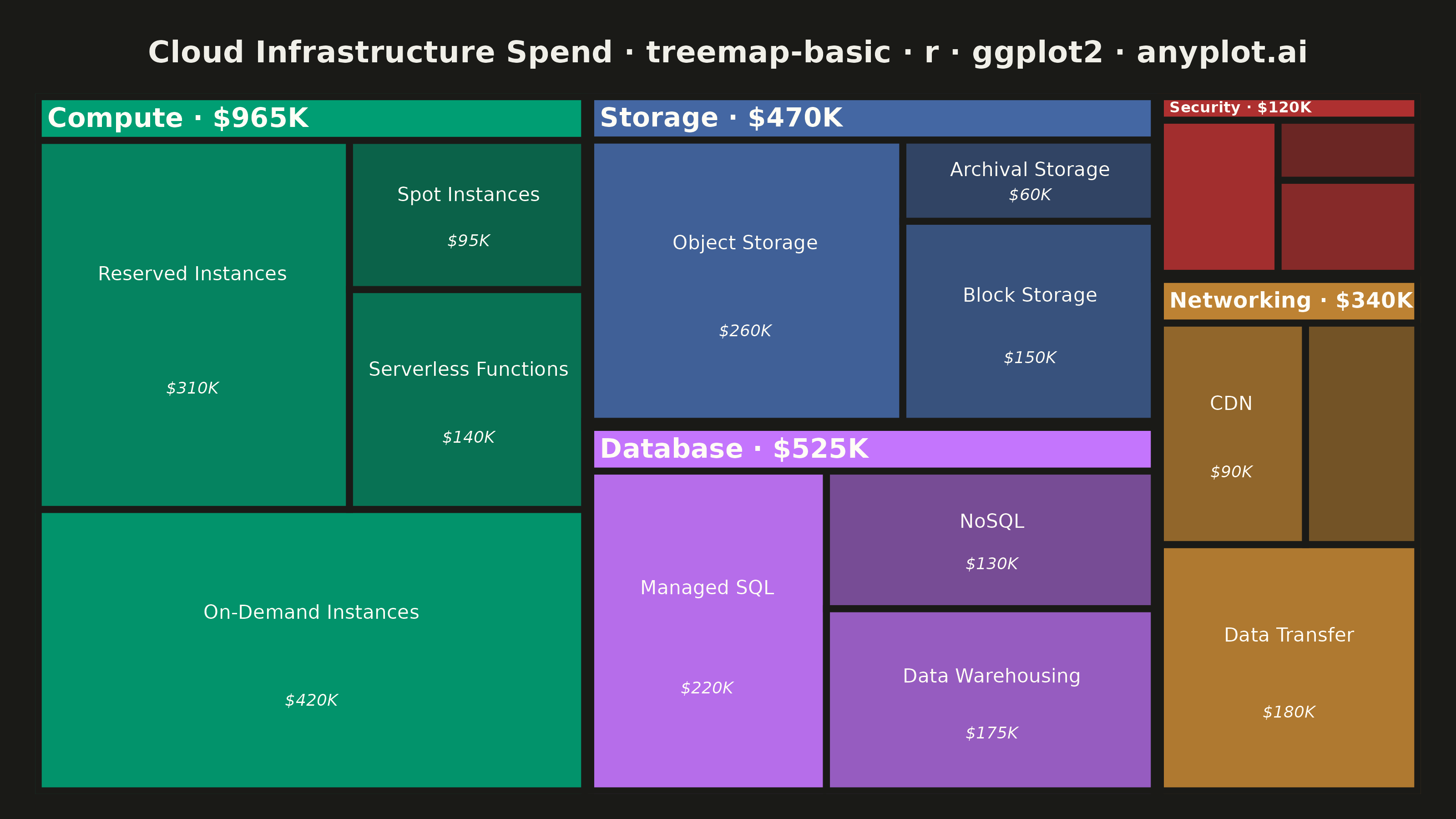
A treemap displaying hierarchical data as nested rectangles, where each rectangle's area is proportional to its value. This visualization excels at showing part-to-whole relationships in hierarchical structures, making it easy to spot large and small items at a glance. Treemaps efficiently use screen space to display large amounts of hierarchical data in a compact form.
#' anyplot.ai
#' treemap-basic: Basic Treemap
#' Library: ggplot2 3.5.1 | R 4.4.1
#' Quality: 91/100 | Created: 2026-08-04

library(ggplot2)
library(dplyr)
library(ragg)

# --- Theme tokens ------------------------------------------------------
THEME       <- Sys.getenv("ANYPLOT_THEME", "light")
PAGE_BG     <- if (THEME == "light") "#FAF8F1" else "#1A1A17"
INK         <- if (THEME == "light") "#1A1A17" else "#F0EFE8"
IMPRINT_PALETTE <- c("#009E73", "#C475FD", "#4467A3", "#BD8233",
                     "#AE3030", "#2ABCCD", "#954477", "#99B314")

# WCAG relative luminance, used to pick readable ink for tile labels
relative_luminance <- function(hex) {
  channel <- grDevices::col2rgb(hex) / 255
  linear <- ifelse(channel <= 0.03928, channel / 12.92, ((channel + 0.055) / 1.055)^2.4)
  sum(c(0.2126, 0.7152, 0.0722) * linear)
}

# Alpha-composite `hex` over `bg_hex` so label ink reflects the tile's
# actual rendered shade (tiles vary alpha to encode hierarchy depth)
blend_hex <- function(hex, bg_hex, alpha) {
  fg <- as.vector(grDevices::col2rgb(hex))
  bg <- as.vector(grDevices::col2rgb(bg_hex))
  blended <- alpha * fg + (1 - alpha) * bg
  grDevices::rgb(blended[1], blended[2], blended[3], maxColorValue = 255)
}

# Squarified treemap layout (Bruls, Huizing & van Wijk, 1999): greedily
# grows rows/columns of tiles that keep aspect ratios close to square,
# recursing into the leftover rectangle after each row is placed.
squarify <- function(values, x, y, w, h) {
  n <- length(values)
  out <- data.frame(xmin = numeric(n), xmax = numeric(n), ymin = numeric(n), ymax = numeric(n))
  if (n == 0) return(out)
  scaled <- values / sum(values) * (w * h)

  worst_ratio <- function(row, side) {
    s <- sum(row)
    max((side^2 * max(row)) / (s^2), (s^2) / (side^2 * min(row)))
  }

  place_row <- function(row_vals, x, y, w, h) {
    side <- min(w, h)
    thickness <- sum(row_vals) / side
    rects <- vector("list", length(row_vals))
    if (w >= h) {
      cy <- y
      for (k in seq_along(row_vals)) {
        seg <- row_vals[k] / thickness
        rects[[k]] <- list(xmin = x, xmax = x + thickness, ymin = cy, ymax = cy + seg)
        cy <- cy + seg
      }
      remainder <- list(x = x + thickness, y = y, w = w - thickness, h = h)
    } else {
      cx <- x
      for (k in seq_along(row_vals)) {
        seg <- row_vals[k] / thickness
        rects[[k]] <- list(xmin = cx, xmax = cx + seg, ymin = y, ymax = y + thickness)
        cx <- cx + seg
      }
      remainder <- list(x = x, y = y + thickness, w = w, h = h - thickness)
    }
    list(rects = rects, remainder = remainder)
  }

  cur_x <- x; cur_y <- y; cur_w <- w; cur_h <- h
  row_vals <- numeric(0); row_idx <- integer(0)
  i <- 1
  while (i <= n || length(row_vals) > 0) {
    if (i <= n) {
      side <- min(cur_w, cur_h)
      trial <- c(row_vals, scaled[i])
      if (length(row_vals) == 0 || worst_ratio(trial, side) <= worst_ratio(row_vals, side)) {
        row_vals <- trial
        row_idx <- c(row_idx, i)
        i <- i + 1
        next
      }
    }
    placed <- place_row(row_vals, cur_x, cur_y, cur_w, cur_h)
    for (k in seq_along(row_idx)) {
      pos <- row_idx[k]
      r <- placed$rects[[k]]
      out$xmin[pos] <- r$xmin; out$xmax[pos] <- r$xmax
      out$ymin[pos] <- r$ymin; out$ymax[pos] <- r$ymax
    }
    rem <- placed$remainder
    cur_x <- rem$x; cur_y <- rem$y; cur_w <- rem$w; cur_h <- rem$h
    row_vals <- numeric(0); row_idx <- integer(0)
  }
  out
}

# --- Data: monthly cloud infrastructure spend ($K) by service category --
leaves <- tibble::tribble(
  ~category,    ~resource,               ~spend,
  "Compute",    "On-Demand Instances",      420,
  "Compute",    "Reserved Instances",       310,
  "Compute",    "Serverless Functions",     140,
  "Compute",    "Spot Instances",            95,
  "Database",   "Managed SQL",              220,
  "Database",   "Data Warehousing",         175,
  "Database",   "NoSQL",                    130,
  "Storage",    "Object Storage",           260,
  "Storage",    "Block Storage",            150,
  "Storage",    "Archival Storage",          60,
  "Networking", "Data Transfer",            180,
  "Networking", "CDN",                       90,
  "Networking", "Load Balancers",            70,
  "Security",   "Identity & Access",         55,
  "Security",   "Threat Detection",          40,
  "Security",   "Key Management",            25
)

# --- Layout: squarify category totals, then subcategories within each ---
DOMAIN_W <- 1600
DOMAIN_H <- 900

cat_totals <- leaves %>%
  group_by(category) %>%
  summarise(total = sum(spend), .groups = "drop") %>%
  arrange(desc(total)) %>%
  mutate(fill_hex = IMPRINT_PALETTE[seq_len(n())])

# A slim header band per category (reserved above its children) holds the
# category name + total, so it never competes for space with leaf labels.
cat_layout <- bind_cols(cat_totals, squarify(cat_totals$total, 0, 0, DOMAIN_W, DOMAIN_H)) %>%
  mutate(
    header_h    = pmin(60, pmax(34, (ymax - ymin) * 0.14)),
    header_label = paste0(category, " · $", total, "K"),
    header_size = pmin(4.2, pmax(2.0, header_h / 16), (xmax - xmin - 20) / (nchar(header_label) * 5.2)),
    header_ink  = ifelse(sapply(fill_hex, relative_luminance) > 0.4, "#1A1A17", "#FFFDF6")
  )

leaf_layout <- bind_rows(lapply(seq_len(nrow(cat_layout)), function(i) {
  cat_row <- cat_layout[i, ]
  sub <- leaves %>% filter(category == cat_row$category) %>% arrange(desc(spend))
  rects <- squarify(sub$spend, cat_row$xmin, cat_row$ymin,
                     cat_row$xmax - cat_row$xmin,
                     (cat_row$ymax - cat_row$header_h) - cat_row$ymin)
  bind_cols(sub, rects) %>% mutate(fill_hex = cat_row$fill_hex)
})) %>%
  group_by(category) %>%
  mutate(
    rank_in_cat = row_number(),
    n_in_cat    = n(),
    tile_alpha  = if (n_in_cat[1] == 1) 0.85 else seq(0.92, 0.55, length.out = n_in_cat[1])[rank_in_cat]
  ) %>%
  ungroup() %>%
  mutate(
    tile_fill  = mapply(function(hex, a) blend_hex(hex, PAGE_BG, a), fill_hex, tile_alpha),
    label_ink  = ifelse(sapply(tile_fill, relative_luminance) > 0.4, "#1A1A17", "#FFFDF6"),
    tile_w     = xmax - xmin,
    tile_h     = ymax - ymin,
    value_label = paste0("$", spend, "K"),
    # Text-width-aware thresholds (~12.5 domain units per char at size 2.7) —
    # narrow tiles omit their label instead of overflowing past their bounds.
    show_name  = tile_w > nchar(resource) * 12.5 & tile_h > 48,
    show_value = show_name & tile_h > 78 & tile_w > nchar(value_label) * 12.5,
    name_y     = ifelse(show_value, (ymin + ymax) / 2 + tile_h * 0.14, (ymin + ymax) / 2)
  )

# --- Title (shrinks to fit when the mandated string runs long) ----------
plot_title  <- "Cloud Infrastructure Spend · treemap-basic · r · ggplot2 · anyplot.ai"
title_ratio <- ifelse(nchar(plot_title) > 67, 67 / nchar(plot_title), 1.0)
title_size  <- max(8, round(12 * title_ratio))

# --- Plot -----------------------------------------------------------------
p <- ggplot() +
  geom_rect(
    data = leaf_layout,
    aes(xmin = xmin, xmax = xmax, ymin = ymin, ymax = ymax, fill = tile_fill),
    color = PAGE_BG, linewidth = 1.3
  ) +
  scale_fill_identity() +
  geom_text(
    data = filter(leaf_layout, show_name),
    aes(x = (xmin + xmax) / 2, y = name_y, label = resource, color = label_ink),
    size = 2.7, lineheight = 0.9
  ) +
  geom_text(
    data = filter(leaf_layout, show_value),
    aes(x = (xmin + xmax) / 2, y = (ymin + ymax) / 2 - tile_h * 0.17,
        label = value_label, color = label_ink),
    size = 2.3, fontface = "italic"
  ) +
  geom_rect(
    data = cat_layout,
    aes(xmin = xmin, xmax = xmax, ymin = ymax - header_h, ymax = ymax, fill = fill_hex),
    color = PAGE_BG, linewidth = 1.3
  ) +
  geom_text(
    data = cat_layout,
    aes(x = xmin + 14, y = ymax - header_h / 2, label = header_label,
        color = header_ink, size = header_size),
    hjust = 0, fontface = "bold"
  ) +
  geom_rect(
    data = cat_layout,
    aes(xmin = xmin, xmax = xmax, ymin = ymin, ymax = ymax),
    fill = NA, color = PAGE_BG, linewidth = 2.4
  ) +
  scale_color_identity() +
  scale_size_identity() +
  scale_x_continuous(limits = c(0, DOMAIN_W), expand = c(0, 0)) +
  scale_y_continuous(limits = c(0, DOMAIN_H), expand = c(0, 0)) +
  labs(title = plot_title) +
  theme_void(base_size = 8) +
  theme(
    plot.background  = element_rect(fill = PAGE_BG, color = PAGE_BG),
    panel.background = element_rect(fill = PAGE_BG, color = NA),
    plot.title       = element_text(color = INK, size = title_size, face = "bold",
                                     hjust = 0.5, margin = margin(t = 6, b = 10)),
    plot.margin      = margin(10, 14, 10, 14)
  )

# --- Save -------------------------------------------------------------------
ggsave(
  filename = sprintf("plot-%s.png", THEME),
  plot     = p,
  device   = ragg::agg_png,
  width    = 8,
  height   = 4.5,
  units    = "in",
  dpi      = 400
)
Runnable source as JSON, for any HTTP client: https://api.anyplot.ai/specs/treemap-basic/ggplot2/code. Any spec id and library id listed in llms-full.txt fit the same URL shape; every URL below is complete and callable.
{
  "spec_id": "treemap-basic",
  "language": "r",
  "library": "ggplot2",
  "page": "https://anyplot.ai/treemap-basic/r/ggplot2",
  "hub": "https://anyplot.ai/treemap-basic",
  "code_json": "https://api.anyplot.ai/specs/treemap-basic/ggplot2/code",
  "spec_json": "https://api.anyplot.ai/specs/treemap-basic",
  "render_light_png": "https://storage.googleapis.com/anyplot-images/plots/treemap-basic/r/ggplot2/plot-light.png",
  "render_dark_png": "https://storage.googleapis.com/anyplot-images/plots/treemap-basic/r/ggplot2/plot-dark.png",
  "quality_score": 91.0,
  "license": "MIT",
  "guide": "https://anyplot.ai/llms.txt"
}
Part of Basic Treemap on anyplot.ai.