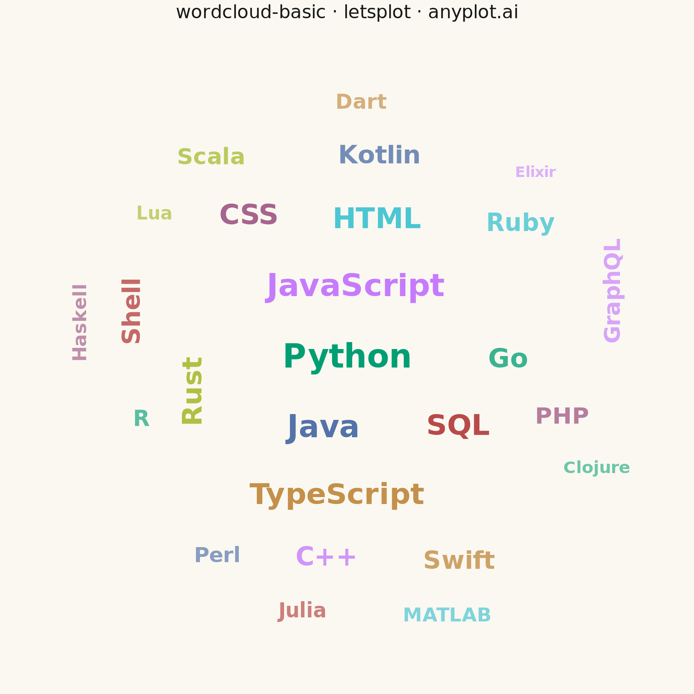
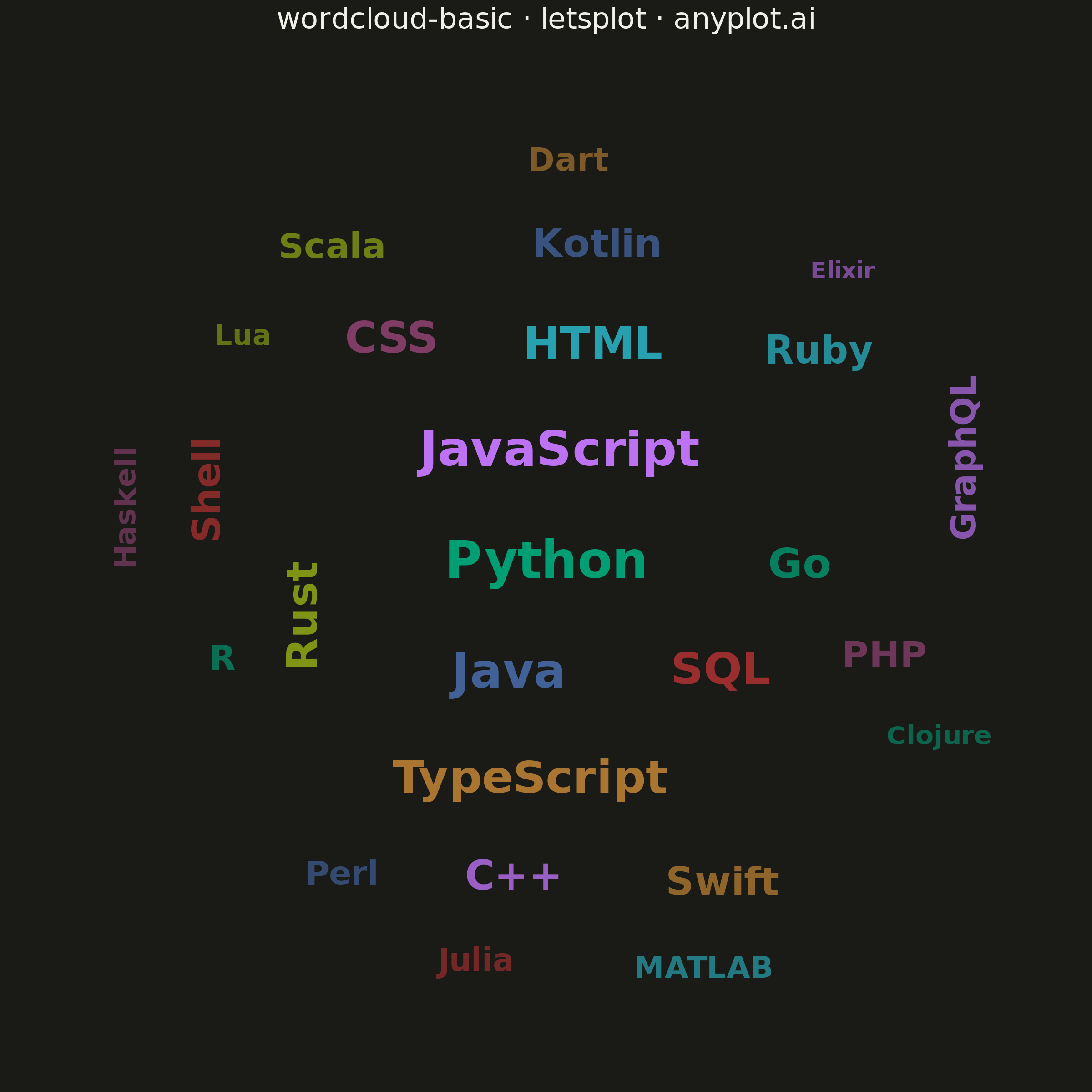
A word cloud displays text data where word size represents frequency or importance. Words are arranged to fill available space, creating a visual summary of text content that highlights prominent terms and patterns. This visualization is ideal for quickly identifying the most common themes or keywords in a body of text.
""" anyplot.ai
wordcloud-basic: Basic Word Cloud
Library: letsplot 4.11.0 | Python 3.13.14
Quality: 85/100 | Updated: 2026-08-04
"""

import math
import os

import numpy as np
import pandas as pd
from lets_plot import (
    LetsPlot,
    aes,
    element_blank,
    element_rect,
    element_text,
    geom_text,
    ggplot,
    ggsize,
    labs,
    layer_tooltips,
    scale_alpha_identity,
    scale_color_manual,
    scale_size_identity,
    scale_x_continuous,
    scale_y_continuous,
    theme,
    theme_void,
)
from lets_plot.export import ggsave


LetsPlot.setup_html()

# Theme tokens
THEME = os.getenv("ANYPLOT_THEME", "light")
PAGE_BG = "#FAF8F1" if THEME == "light" else "#1A1A17"
INK = "#1A1A17" if THEME == "light" else "#F0EFE8"
INK_SOFT = "#4A4A44" if THEME == "light" else "#B8B7B0"

# Imprint palette (first series always #009E73)
IMPRINT = ["#009E73", "#C475FD", "#4467A3", "#BD8233", "#AE3030", "#2ABCCD", "#954477", "#99B314"]

# Data - Programming language popularity
np.random.seed(42)
words_data = {
    "Python": 100,
    "JavaScript": 92,
    "Java": 85,
    "TypeScript": 78,
    "SQL": 75,
    "HTML": 70,
    "CSS": 68,
    "Rust": 62,
    "Go": 58,
    "C++": 55,
    "Kotlin": 52,
    "Swift": 50,
    "Shell": 48,
    "Ruby": 45,
    "PHP": 42,
    "Scala": 38,
    "R": 35,
    "Perl": 32,
    "Dart": 30,
    "Julia": 28,
    "MATLAB": 26,
    "Haskell": 24,
    "Lua": 22,
    "Clojure": 20,
    "Elixir": 18,
    "GraphQL": 35,
}

words = list(words_data.keys())
frequencies = list(words_data.values())

# Sort by frequency (largest first for better placement)
sorted_indices = np.argsort(frequencies)[::-1]
words = [words[i] for i in sorted_indices]
frequencies = [frequencies[i] for i in sorted_indices]

# Canvas dimensions (data-space, independent of the exported pixel size) -
# square domain so the naturally circular/blob-shaped spiral fills the frame
# evenly on all sides (landscape left large empty side margins)
canvas_width = 150
canvas_height = 150

# Scale font sizes for readability (mm, geom_text units) - floor raised so the
# smallest-frequency words stay legible once scaled down to mobile widths
min_freq, max_freq = min(frequencies), max(frequencies)
min_size, max_size = 6.5, 14

sizes = []
for freq in frequencies:
    normalized = (freq - min_freq) / (max_freq - min_freq)
    size = min_size + (normalized**0.6) * (max_size - min_size)
    sizes.append(size)

# Fade lower-frequency words slightly so the eye lands on the dominant terms first
alphas = [0.55 + 0.45 * ((freq - min_freq) / (max_freq - min_freq)) for freq in frequencies]

# Vertical rotation for a subset of words (skip the top 3 focal terms) - a
# lets-plot geom_text `angle` aesthetic, the classic word-cloud variety cue
angles = [90 if (i >= 3 and i % 5 == 2) else 0 for i in range(len(words))]

# Spiral word placement with collision detection (rotation-aware bounding box)
placed = []
positions_x = []
positions_y = []
char_width_ratio = 0.62

for word, size, angle in zip(words, sizes, angles, strict=True):
    raw_width = len(word) * size * char_width_ratio
    raw_height = size * 1.05
    word_width, word_height = (raw_height, raw_width) if angle == 90 else (raw_width, raw_height)

    t = 0
    step = 0.08
    max_iterations = 4000
    placed_word = False

    while t < max_iterations and not placed_word:
        r = 0.1 + t * 0.08
        theta = t * 0.35
        x = canvas_width / 2 + r * math.cos(theta) * 0.95
        y = canvas_height / 2 + r * math.sin(theta)

        margin = 3
        if (
            x - word_width / 2 < margin
            or x + word_width / 2 > canvas_width - margin
            or y - word_height / 2 < margin
            or y + word_height / 2 > canvas_height - margin
        ):
            t += step
            continue

        collision = False
        padding = 1.6
        for px, py, pw, ph in placed:
            if abs(x - px) < (word_width / 2 + pw / 2 + padding) and abs(y - py) < (word_height / 2 + ph / 2 + padding):
                collision = True
                break

        if not collision:
            placed.append((x, y, word_width, word_height))
            positions_x.append(x)
            positions_y.append(y)
            placed_word = True
        else:
            t += step

    if not placed_word:
        positions_x.append(None)
        positions_y.append(None)

# Build dataframe with placed words
df_data = []
for word, freq, size, angle, alpha, x, y in zip(
    words, frequencies, sizes, angles, alphas, positions_x, positions_y, strict=True
):
    if x is not None and y is not None:
        df_data.append({"word": word, "frequency": freq, "size": size, "angle": angle, "alpha": alpha, "x": x, "y": y})

df = pd.DataFrame(df_data)

# Assign Imprint colors to words
df["color"] = [IMPRINT[i % len(IMPRINT)] for i in range(len(df))]

# Plot with theme-adaptive chrome
anyplot_theme = theme(
    plot_background=element_rect(fill=PAGE_BG, color=PAGE_BG),
    panel_background=element_rect(fill=PAGE_BG, color=PAGE_BG),
    plot_title=element_text(size=16, color=INK, hjust=0.5),
    legend_position="none",
    axis_title=element_blank(),
    axis_text=element_blank(),
)

word_tooltips = layer_tooltips().title("@word").line("Frequency|@frequency")

plot = (
    ggplot(df, aes(x="x", y="y", label="word", size="size", color="color", angle="angle", alpha="alpha"))
    + geom_text(fontface="bold", tooltips=word_tooltips)
    + scale_size_identity()
    + scale_alpha_identity()
    + scale_color_manual(values=df["color"].unique(), guide="none")
    + scale_x_continuous(limits=(0, canvas_width), expand=[0, 0])
    + scale_y_continuous(limits=(0, canvas_height), expand=[0, 0])
    + labs(title="wordcloud-basic · letsplot · anyplot.ai")
    + theme_void()
    + anyplot_theme
    + ggsize(600, 600)
)

# Save
ggsave(plot, f"plot-{THEME}.png", path=".", scale=4)
ggsave(plot, f"plot-{THEME}.html", path=".")
Runnable source as JSON, for any HTTP client: https://api.anyplot.ai/specs/wordcloud-basic/letsplot/code. Any spec id and library id listed in llms-full.txt fit the same URL shape; every URL below is complete and callable.
{
  "spec_id": "wordcloud-basic",
  "language": "python",
  "library": "letsplot",
  "page": "https://anyplot.ai/wordcloud-basic/python/letsplot",
  "hub": "https://anyplot.ai/wordcloud-basic",
  "code_json": "https://api.anyplot.ai/specs/wordcloud-basic/letsplot/code",
  "spec_json": "https://api.anyplot.ai/specs/wordcloud-basic",
  "render_light_png": "https://storage.googleapis.com/anyplot-images/plots/wordcloud-basic/python/letsplot/plot-light.png",
  "render_dark_png": "https://storage.googleapis.com/anyplot-images/plots/wordcloud-basic/python/letsplot/plot-dark.png",
  "interactive_light_html": "https://storage.googleapis.com/anyplot-images/plots/wordcloud-basic/python/letsplot/plot-light.html",
  "interactive_dark_html": "https://storage.googleapis.com/anyplot-images/plots/wordcloud-basic/python/letsplot/plot-dark.html",
  "quality_score": 85.0,
  "license": "MIT",
  "guide": "https://anyplot.ai/llms.txt"
}
Part of Basic Word Cloud on anyplot.ai.