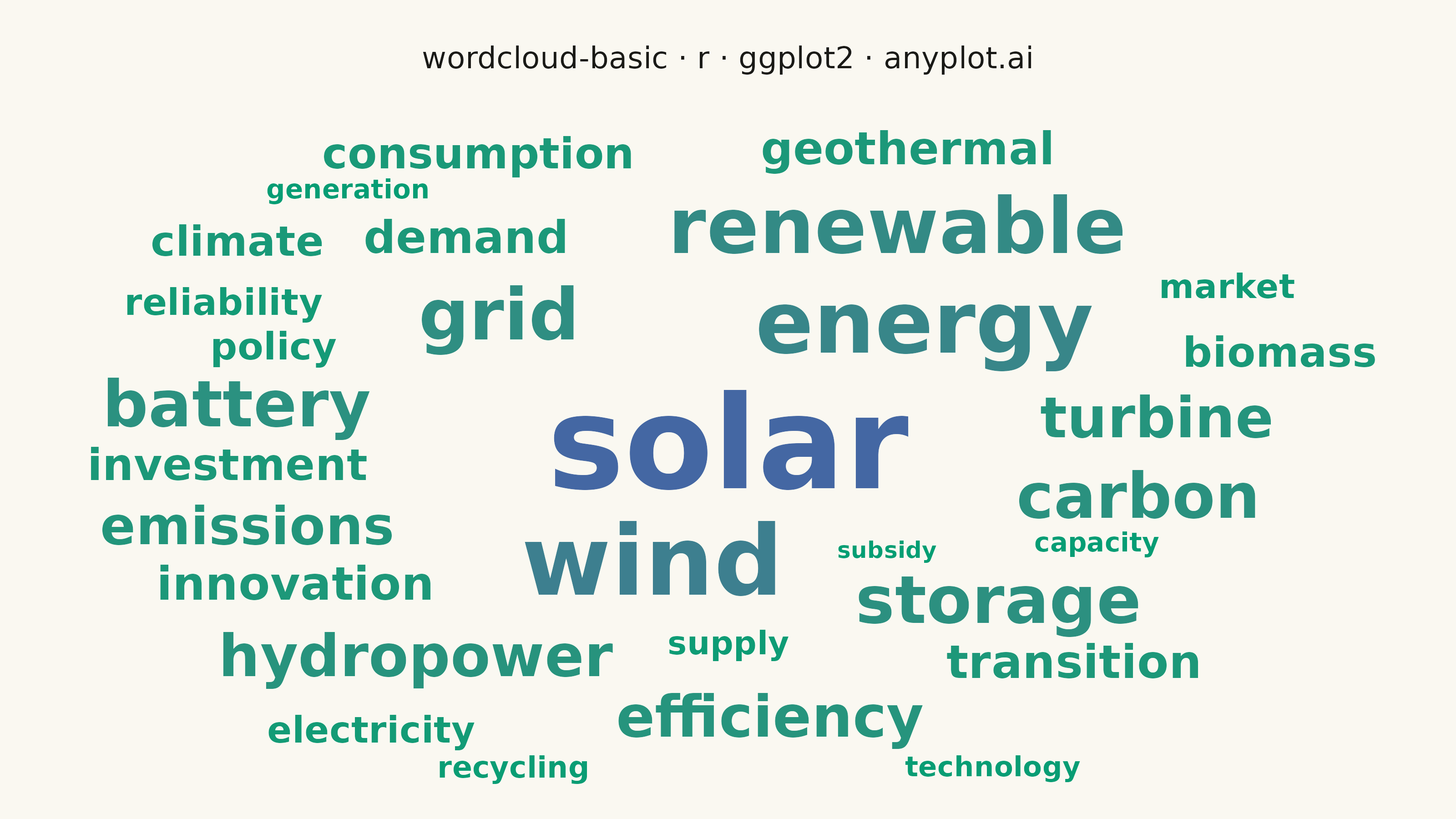
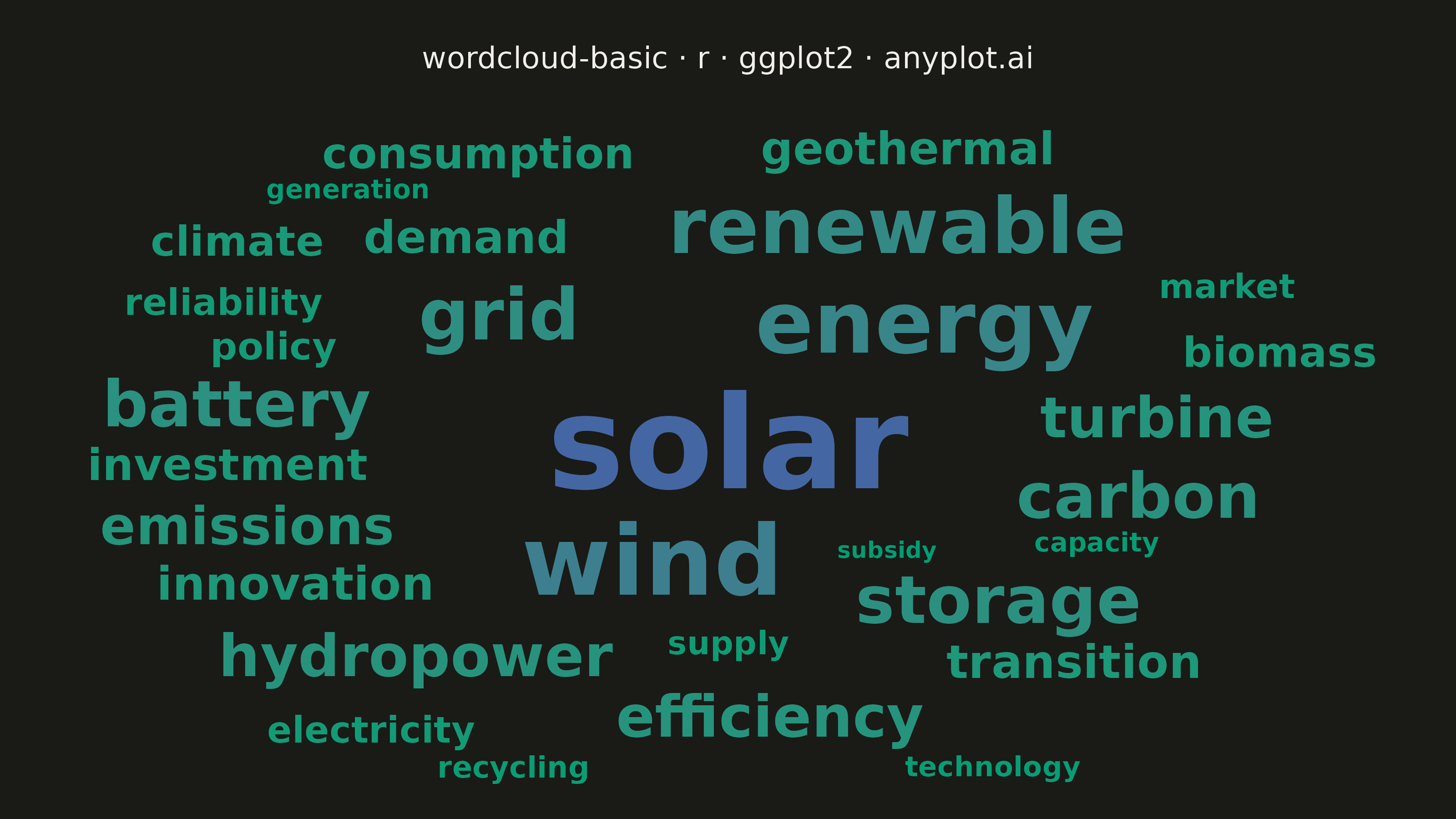
A word cloud displays text data where word size represents frequency or importance. Words are arranged to fill available space, creating a visual summary of text content that highlights prominent terms and patterns. This visualization is ideal for quickly identifying the most common themes or keywords in a body of text.
#' anyplot.ai
#' wordcloud-basic: Basic Word Cloud
#' Library: ggplot2 3.5.1 | R 4.4.1
#' Quality: 91/100 | Created: 2026-08-04

library(ggplot2)
library(tibble)
library(ragg)

set.seed(42)

# --- Theme tokens -------------------------------------------------------------
THEME       <- Sys.getenv("ANYPLOT_THEME", "light")
PAGE_BG     <- if (THEME == "light") "#FAF8F1" else "#1A1A17"
INK         <- if (THEME == "light") "#1A1A17" else "#F0EFE8"
IMPRINT_PALETTE <- c("#009E73", "#C475FD", "#4467A3", "#BD8233",
                     "#AE3030", "#2ABCCD", "#954477", "#99B314")
BRAND <- IMPRINT_PALETTE[1]

# --- Data: term frequencies from a renewable-energy report scan ---------------
terms <- c(
  "solar", "wind", "energy", "renewable", "grid", "battery", "storage",
  "efficiency", "carbon", "emissions", "turbine", "hydropower", "biomass",
  "geothermal", "investment", "innovation", "climate", "capacity",
  "generation", "transition", "policy", "technology", "electricity",
  "consumption", "demand", "supply", "market", "subsidy", "reliability",
  "recycling"
)
rank_order <- seq_along(terms)
base_freq  <- 150 / rank_order^0.65
frequency  <- pmax(round(base_freq + rnorm(length(terms), mean = 0, sd = 4)), 5)

word_freq <- tibble(word = terms, frequency = frequency)
word_freq <- word_freq[order(-word_freq$frequency), ]

# Font size scales with sqrt(frequency) so rendered AREA (not height) tracks
# term frequency, matching how the eye compares word-cloud prominence.
size_min <- 3.2
size_max <- 18
freq_sqrt <- sqrt(word_freq$frequency)
word_freq$text_size <- size_min + (freq_sqrt - min(freq_sqrt)) /
  diff(range(freq_sqrt)) * (size_max - size_min)

# --- Layout: box-bounded spiral placement with rectangle collision ------------
# geom_text's `size` aesthetic is in millimetres, so the layout below works
# directly in millimetres too (1 coordinate unit = 1 mm) and the panel is
# rendered at that exact physical scale via coord_fixed(ratio = 1) below —
# this keeps the hand-measured bounding boxes true to the rendered glyphs.
# Bounding-box multipliers are calibrated from grid::grobWidth/grobHeight on
# the bold sans face actually used for geom_text (see dev notes: width per
# char ranges ~0.55-0.68x fontsize, height ~0.735x fontsize; padded up here
# for a safety margin against overlap).
half_w_per_char <- 0.35
half_h_factor   <- 0.42
box_half_w <- 86   # mm — half-width of the placement box (172mm total)
box_half_h <- 44   # mm — half-height of the placement box (88mm total)
x_stretch  <- box_half_w / box_half_h

n_words  <- nrow(word_freq)
placed_x <- numeric(n_words)
placed_y <- numeric(n_words)
placed_hw <- numeric(n_words)
placed_hh <- numeric(n_words)
max_radius <- sqrt(box_half_w^2 + box_half_h^2)

# Fallback grid, closest-to-center first, for words the spiral walk can't
# place within its step budget (a spiral path only samples one point per
# radius, so it can miss small pockets of free space that a grid catches).
grid_x <- seq(-box_half_w, box_half_w, by = 1)
grid_y <- seq(-box_half_h, box_half_h, by = 1)
fallback_grid <- expand.grid(x = grid_x, y = grid_y)
fallback_grid <- fallback_grid[order(sqrt((fallback_grid$x / x_stretch)^2 + fallback_grid$y^2)), ]

for (i in seq_len(n_words)) {
  fs <- word_freq$text_size[i]
  half_w <- nchar(word_freq$word[i]) * fs * half_w_per_char
  half_h <- fs * half_h_factor
  placed <- FALSE

  if (i == 1) {
    cx <- 0
    cy <- 0
    placed <- TRUE
  } else {
    theta <- 0
    radius <- 0
    step <- 0
    repeat {
      cx <- radius * cos(theta) * x_stretch
      cy <- radius * sin(theta)

      in_box <- (abs(cx) + half_w <= box_half_w) && (abs(cy) + half_h <= box_half_h)
      overlap <- !in_box
      if (in_box) {
        for (j in seq_len(i - 1)) {
          dx <- abs(cx - placed_x[j])
          dy <- abs(cy - placed_y[j])
          if (dx < (half_w + placed_hw[j]) * 1.06 && dy < (half_h + placed_hh[j]) * 1.15) {
            overlap <- TRUE
            break
          }
        }
      }
      if (!overlap) {
        placed <- TRUE
        break
      }

      theta <- theta + 0.12
      radius <- min(radius + 0.18, max_radius)
      step <- step + 1
      if (step > 8000) break
    }
  }

  if (!placed) {
    for (k in seq_len(nrow(fallback_grid))) {
      gx <- fallback_grid$x[k]
      gy <- fallback_grid$y[k]
      if (abs(gx) + half_w > box_half_w || abs(gy) + half_h > box_half_h) next
      overlap <- FALSE
      for (j in seq_len(i - 1)) {
        dx <- abs(gx - placed_x[j])
        dy <- abs(gy - placed_y[j])
        if (dx < (half_w + placed_hw[j]) * 1.06 && dy < (half_h + placed_hh[j]) * 1.15) {
          overlap <- TRUE
          break
        }
      }
      if (!overlap) {
        cx <- gx
        cy <- gy
        placed <- TRUE
        break
      }
    }
  }

  placed_x[i] <- cx
  placed_y[i] <- cy
  placed_hw[i] <- half_w
  placed_hh[i] <- half_h
}

word_freq$x <- placed_x
word_freq$y <- placed_y

# --- Plot -----------------------------------------------------------------
plot_title <- "wordcloud-basic · r · ggplot2 · anyplot.ai"
title_ratio <- if (nchar(plot_title) > 67) 67 / nchar(plot_title) else 1.0
title_size <- round(12 * title_ratio)

p <- ggplot(word_freq, aes(x = x, y = y, label = word,
                            size = text_size, color = frequency)) +
  geom_text(fontface = "bold", family = "sans") +
  scale_size_identity() +
  scale_color_gradient(low = BRAND, high = "#4467A3", guide = "none") +
  scale_x_continuous(limits = c(-box_half_w, box_half_w), expand = c(0, 0)) +
  scale_y_continuous(limits = c(-box_half_h, box_half_h), expand = c(0, 0)) +
  coord_fixed(ratio = 1, clip = "off") +
  labs(title = plot_title) +
  theme_void(base_size = 8) +
  theme(
    plot.background = element_rect(fill = PAGE_BG, color = PAGE_BG),
    plot.title = element_text(color = INK, size = title_size, hjust = 0.5,
                               margin = margin(b = 10)),
    plot.margin = margin(t = 16, r = 24, b = 12, l = 24)
  )

# --- Save -------------------------------------------------------------------
ggsave(
  filename = sprintf("plot-%s.png", THEME),
  plot     = p,
  device   = ragg::agg_png,
  width    = 8,
  height   = 4.5,
  units    = "in",
  dpi      = 400
)
Runnable source as JSON, for any HTTP client: https://api.anyplot.ai/specs/wordcloud-basic/ggplot2/code. Any spec id and library id listed in llms-full.txt fit the same URL shape; every URL below is complete and callable.
{
  "spec_id": "wordcloud-basic",
  "language": "r",
  "library": "ggplot2",
  "page": "https://anyplot.ai/wordcloud-basic/r/ggplot2",
  "hub": "https://anyplot.ai/wordcloud-basic",
  "code_json": "https://api.anyplot.ai/specs/wordcloud-basic/ggplot2/code",
  "spec_json": "https://api.anyplot.ai/specs/wordcloud-basic",
  "render_light_png": "https://storage.googleapis.com/anyplot-images/plots/wordcloud-basic/r/ggplot2/plot-light.png",
  "render_dark_png": "https://storage.googleapis.com/anyplot-images/plots/wordcloud-basic/r/ggplot2/plot-dark.png",
  "quality_score": 91.0,
  "license": "MIT",
  "guide": "https://anyplot.ai/llms.txt"
}
Part of Basic Word Cloud on anyplot.ai.