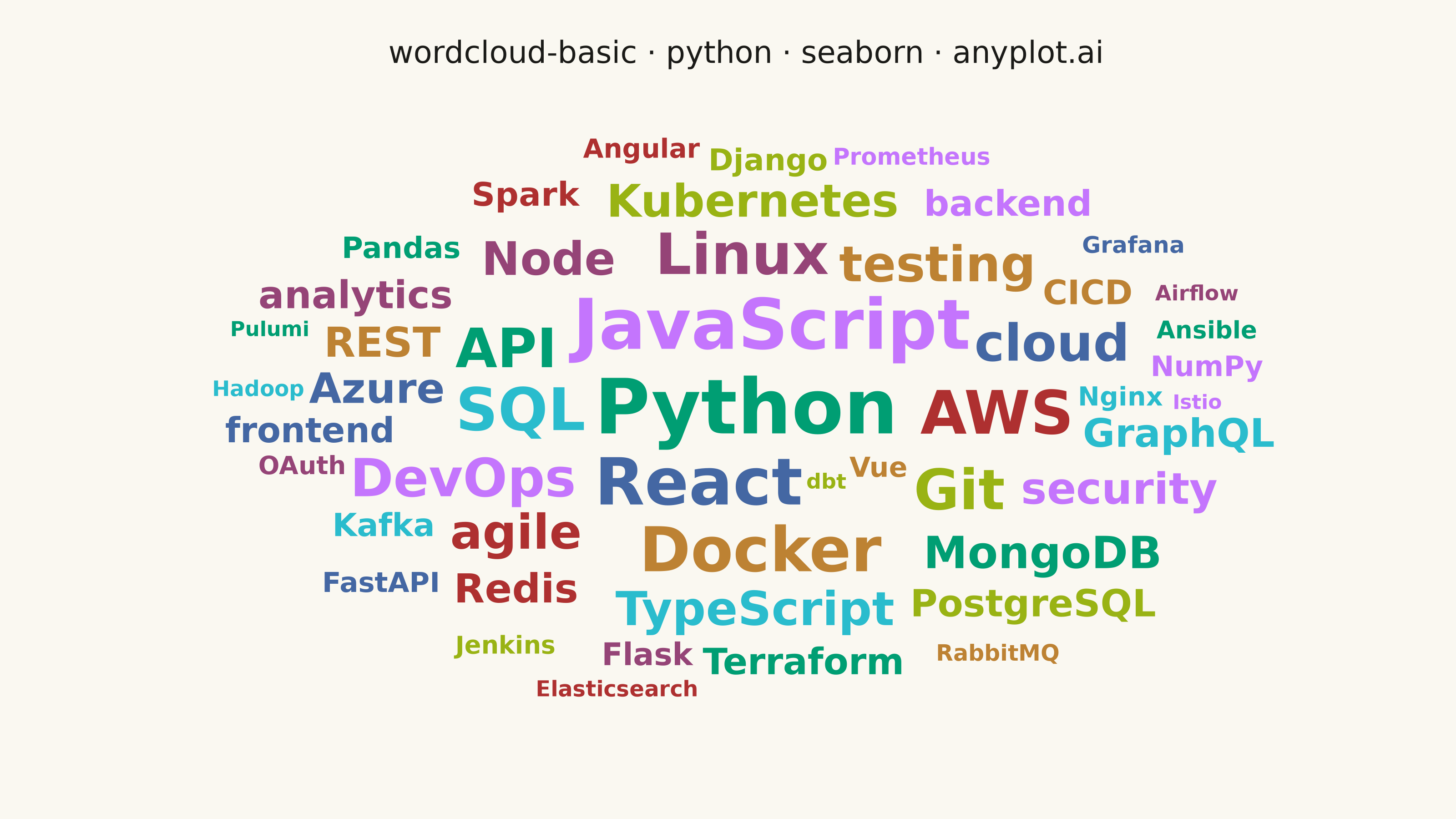
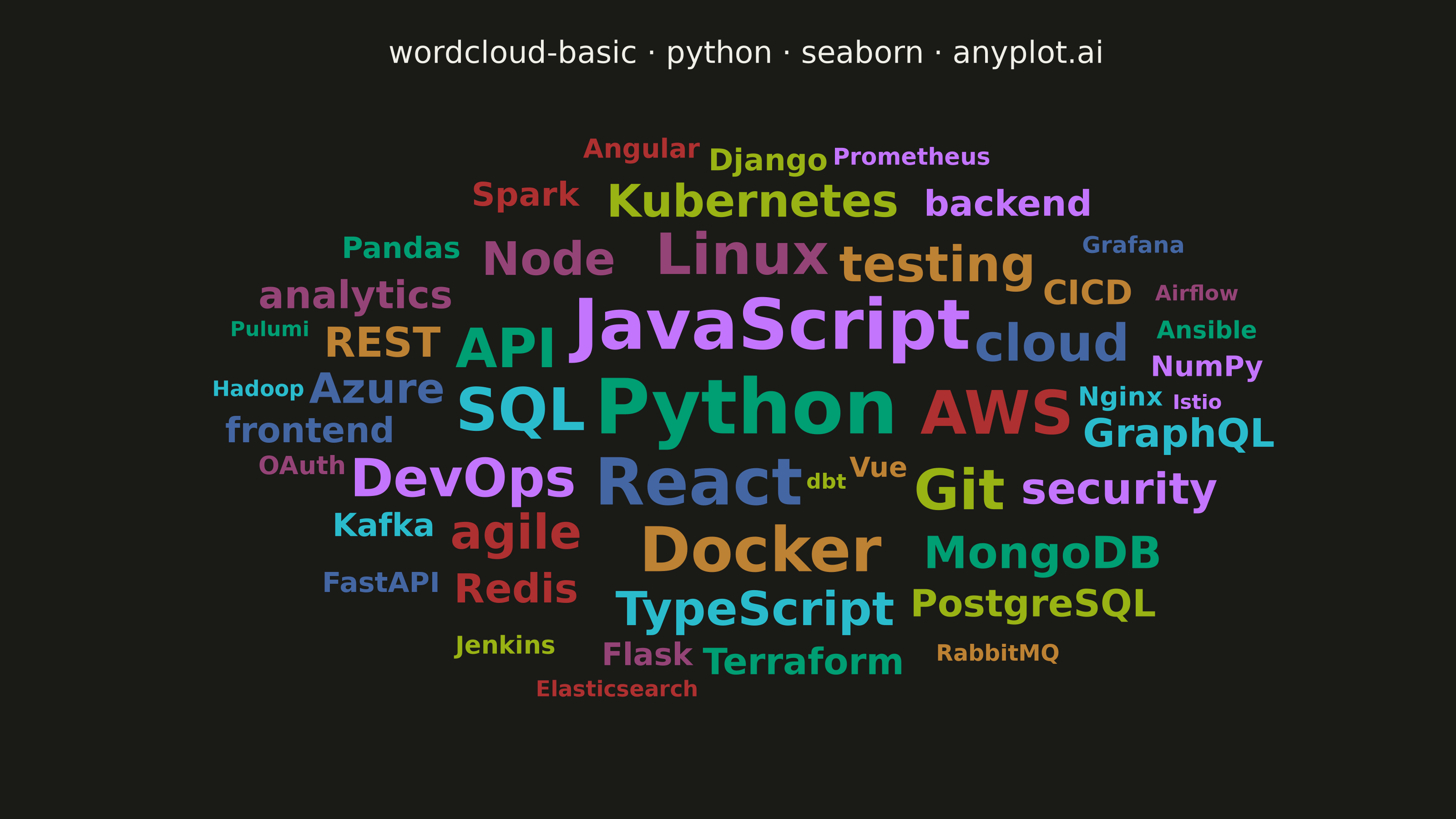
A word cloud displays text data where word size represents frequency or importance. Words are arranged to fill available space, creating a visual summary of text content that highlights prominent terms and patterns. This visualization is ideal for quickly identifying the most common themes or keywords in a body of text.
""" anyplot.ai
wordcloud-basic: Basic Word Cloud
Library: seaborn 0.13.2 | Python 3.13.14
Quality: 86/100 | Updated: 2026-08-04
"""

import os

import matplotlib.pyplot as plt
import numpy as np
import seaborn as sns


# Theme tokens
THEME = os.getenv("ANYPLOT_THEME", "light")
PAGE_BG = "#FAF8F1" if THEME == "light" else "#1A1A17"
INK = "#1A1A17" if THEME == "light" else "#F0EFE8"

# Imprint palette — canonical order, first series always #009E73 — built via
# sns.color_palette() so seaborn validates/normalizes the hex values instead of
# using the raw list directly.
IMPRINT_PALETTE = sns.color_palette(
    ["#009E73", "#C475FD", "#4467A3", "#BD8233", "#AE3030", "#2ABCCD", "#954477", "#99B314"]
).as_hex()

sns.set_theme(
    style="white",
    rc={"figure.facecolor": PAGE_BG, "axes.facecolor": PAGE_BG, "font.family": "sans-serif", "text.color": INK},
)
# Drives the title's font size below (plt.rcParams["axes.titlesize"]) so the
# text scale is governed by seaborn's context system, not a bare literal.
sns.set_context("notebook", font_scale=1.0)

# Data - tech-skill mentions from a developer survey (frequency = respondent count).
# Brand/product names and acronyms keep their established casing (Python, AWS, SQL,
# ...); generic descriptive terms are lowercased per the spec's preprocessing note.
word_frequencies = {
    "Python": 180,
    "JavaScript": 160,
    "React": 145,
    "Docker": 135,
    "AWS": 130,
    "SQL": 125,
    "Linux": 120,
    "Git": 115,
    "API": 110,
    "DevOps": 105,
    "cloud": 100,
    "testing": 95,
    "agile": 90,
    "TypeScript": 87,
    "Node": 84,
    "Kubernetes": 81,
    "MongoDB": 78,
    "security": 75,
    "Azure": 72,
    "REST": 69,
    "Redis": 66,
    "GraphQL": 63,
    "analytics": 60,
    "PostgreSQL": 57,
    "Terraform": 54,
    "backend": 51,
    "frontend": 48,
    "CICD": 45,
    "Spark": 42,
    "Kafka": 39,
    "Flask": 36,
    "Django": 33,
    "Pandas": 30,
    "NumPy": 28,
    "FastAPI": 26,
    "Vue": 24,
    "Angular": 22,
    "Nginx": 20,
    "OAuth": 18,
    "Jenkins": 16,
    "Ansible": 14,
    "Prometheus": 12,
    "Grafana": 10,
    "RabbitMQ": 8,
    "Elasticsearch": 7,
    "Hadoop": 6,
    "Airflow": 5,
    "dbt": 4,
    "Pulumi": 3,
    "Istio": 2,
}

# Sort largest-frequency-first so big words claim the center before small ones fill the gaps
words = sorted(word_frequencies, key=word_frequencies.get, reverse=True)
frequencies = np.array([word_frequencies[w] for w in words], dtype=float)

min_freq, max_freq = frequencies.min(), frequencies.max()
font_sizes = 8 + (frequencies - min_freq) / (max_freq - min_freq) * 22

# Plot — collision-aware spiral placement (checks each word's real rendered
# bounding box against every word already placed, instead of a fixed spiral
# offset that lets neighbors overlap)
fig, ax = plt.subplots(figsize=(8, 4.5), dpi=400, facecolor=PAGE_BG)
ax.set_facecolor(PAGE_BG)

x_half, y_half = 1.0, 0.5625
ax.set_xlim(-x_half, x_half)
ax.set_ylim(-y_half, y_half)
ax.axis("off")

fig.canvas.draw()
renderer = fig.canvas.get_renderer()
inv = ax.transData.inverted()


def half_extent_data(word, fontsize):
    probe = ax.text(0, 0, word, fontsize=fontsize, fontweight="bold", ha="center", va="center", alpha=0)
    bbox = probe.get_window_extent(renderer=renderer)
    probe.remove()
    (x0, y0), (x1, y1) = inv.transform([(bbox.x0, bbox.y0), (bbox.x1, bbox.y1)])
    return (x1 - x0) / 2, (y1 - y0) / 2


def collides(x, y, hw, hh, pad, boxes):
    x0, y0, x1, y1 = x - hw - pad, y - hh - pad, x + hw + pad, y + hh + pad
    for bx0, by0, bx1, by1 in boxes:
        if x0 < bx1 and x1 > bx0 and y0 < by1 and y1 > by0:
            return True
    return False


golden_angle = np.pi * (3 - np.sqrt(5))
max_steps = 900
# Normalized radius up to sqrt(2) so the spiral (scaled independently per axis
# below) reaches the canvas corners instead of tracing an inscribed ellipse.
spiral_scale = np.sqrt(2) / np.sqrt(max_steps)
placed_boxes = []
pad = 0.005

for idx, (word, target_fontsize) in enumerate(zip(words, font_sizes, strict=True)):
    color = IMPRINT_PALETTE[idx % len(IMPRINT_PALETTE)]
    fontsize = target_fontsize
    # A word that can't find a free spot at its target size shrinks and
    # retries, instead of falling back to a fixed spot where it would
    # stack on top of whatever was already placed there.
    for _shrink_attempt in range(6):
        hw, hh = half_extent_data(word, fontsize)
        x, y, found = 0.0, 0.0, False
        for step in range(max_steps):
            angle = step * golden_angle
            norm_radius = spiral_scale * np.sqrt(step)
            cand_x = np.clip(norm_radius * np.cos(angle) * x_half, -x_half + hw, x_half - hw)
            cand_y = np.clip(norm_radius * np.sin(angle) * y_half, -y_half + hh, y_half - hh)
            if not collides(cand_x, cand_y, hw, hh, pad, placed_boxes):
                x, y, found = cand_x, cand_y, True
                break
        if found:
            break
        fontsize *= 0.82
    placed_boxes.append((x - hw, y - hh, x + hw, y + hh))
    ax.text(x, y, word, fontsize=fontsize, fontweight="bold", ha="center", va="center", color=color)

ax.set_title(
    "wordcloud-basic · python · seaborn · anyplot.ai",
    fontsize=plt.rcParams["axes.titlesize"],
    fontweight="medium",
    color=INK,
    pad=14,
)

plt.savefig(f"plot-{THEME}.png", dpi=400, facecolor=PAGE_BG)
Runnable source as JSON, for any HTTP client: https://api.anyplot.ai/specs/wordcloud-basic/seaborn/code. Any spec id and library id listed in llms-full.txt fit the same URL shape; every URL below is complete and callable.
{
  "spec_id": "wordcloud-basic",
  "language": "python",
  "library": "seaborn",
  "page": "https://anyplot.ai/wordcloud-basic/python/seaborn",
  "hub": "https://anyplot.ai/wordcloud-basic",
  "code_json": "https://api.anyplot.ai/specs/wordcloud-basic/seaborn/code",
  "spec_json": "https://api.anyplot.ai/specs/wordcloud-basic",
  "render_light_png": "https://storage.googleapis.com/anyplot-images/plots/wordcloud-basic/python/seaborn/plot-light.png",
  "render_dark_png": "https://storage.googleapis.com/anyplot-images/plots/wordcloud-basic/python/seaborn/plot-dark.png",
  "quality_score": 86.0,
  "license": "MIT",
  "guide": "https://anyplot.ai/llms.txt"
}
Part of Basic Word Cloud on anyplot.ai.