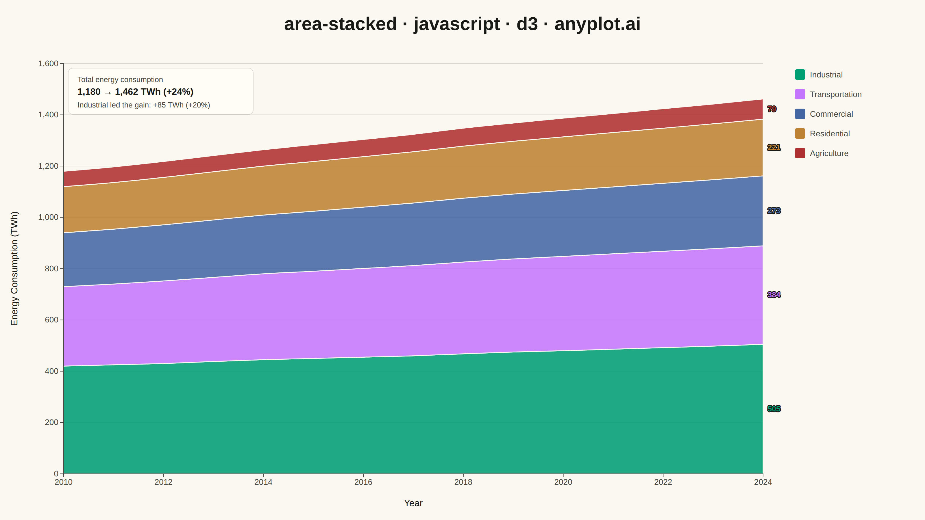
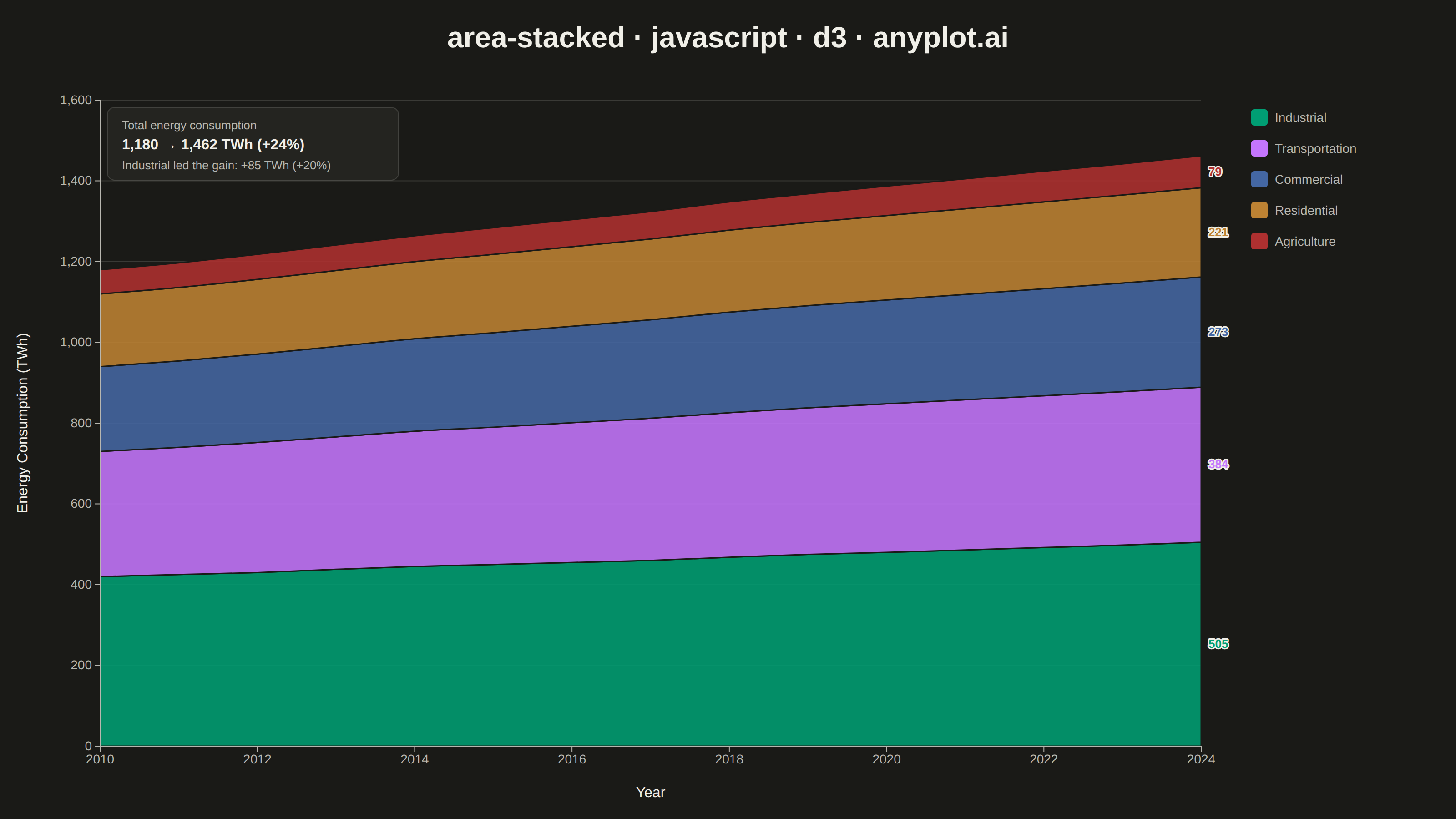
The same plot in 14 other libraries — JavaScript: Chart.js, Apache ECharts, Highcharts, MUI X Charts; Python: Altair, Bokeh, lets-plot, Matplotlib, Plotly, plotnine, Pygal, Seaborn; R: ggplot2; Julia: Makie.jl. Compare all 15 side by side: Stacked Area Chart in Python, R, Julia and JavaScript.
A stacked area chart displays multiple data series as areas stacked on top of each other, with each series starting where the previous one ends. This visualization emphasizes both individual contributions and cumulative totals over a continuous axis (typically time). It is ideal for showing how parts contribute to a whole while tracking changes over time, making patterns of composition and overall trends immediately visible.
// anyplot.ai
// area-stacked: Stacked Area Chart
// Library: d3 7.9.0 | JavaScript 22.23.2
// Quality: 94/100 | Created: 2026-08-17

const t = window.ANYPLOT_TOKENS;
const { width, height } = window.ANYPLOT_SIZE;
const margin = { top: 110, right: 280, bottom: 80, left: 110 };
const iw = width - margin.left - margin.right;
const ih = height - margin.top - margin.bottom;

// --- Data: Germany energy consumption by sector, 2010-2024 (TWh) -----------
// Ordered largest series first so it lands at the base of the stack.
const sectors = [
  { key: "industrial", label: "Industrial",
    values: [420, 425, 430, 438, 445, 450, 455, 460, 468, 475, 480, 486, 492, 498, 505] },
  { key: "transportation", label: "Transportation",
    values: [310, 315, 322, 328, 335, 340, 346, 352, 358, 363, 368, 372, 376, 380, 384] },
  { key: "commercial", label: "Commercial",
    values: [210, 214, 219, 224, 229, 234, 239, 244, 249, 253, 257, 261, 265, 269, 273] },
  { key: "residential", label: "Residential",
    values: [180, 182, 185, 188, 191, 194, 197, 200, 203, 206, 209, 212, 215, 218, 221] },
  { key: "agriculture", label: "Agriculture",
    values: [60, 61, 62, 63, 64, 66, 67, 68, 70, 71, 73, 74, 76, 77, 79] },
];
const years = d3.range(2010, 2025);
const data = years.map((year, i) => {
  const row = { year };
  sectors.forEach((s) => (row[s.key] = s.values[i]));
  return row;
});
const keys = sectors.map((s) => s.key);
const series = d3.stack().keys(keys)(data);

// --- Scales -------------------------------------------------------------
const x = d3.scaleLinear().domain(d3.extent(years)).range([0, iw]);
const yMax = d3.max(series, (layer) => d3.max(layer, (d) => d[1]));
const y = d3.scaleLinear().domain([0, yMax]).nice().range([ih, 0]);
const color = d3.scaleOrdinal().domain(keys).range(t.palette);

// --- SVG mount ------------------------------------------------------------
const svg = d3.select("#container").append("svg").attr("width", width).attr("height", height);
const g = svg.append("g").attr("transform", `translate(${margin.left},${margin.top})`);

// --- Gridlines (y-axis only) ------------------------------------------------
g.append("g")
  .call(d3.axisLeft(y).ticks(6).tickSize(-iw).tickFormat(""))
  .selectAll("line")
  .attr("stroke", t.grid);
g.select(".domain").remove();

// --- Areas ------------------------------------------------------------------
const area = d3
  .area()
  .x((d) => x(d.data.year))
  .y0((d) => y(d[0]))
  .y1((d) => y(d[1]))
  .curve(d3.curveMonotoneX);

g.selectAll("path.layer")
  .data(series)
  .join("path")
  .attr("class", "layer")
  .attr("fill", (d) => color(d.key))
  .attr("fill-opacity", 0.88)
  .attr("stroke", t.pageBg)
  .attr("stroke-width", 1.5)
  .attr("d", area);

// --- Direct end-of-series value labels (color-matched to each layer) --------
// Distinctive-D3 touch: read each layer's final band height straight off the
// stack datum instead of leaning on the legend alone for value lookup.
const lastIdx = data.length - 1;
g.selectAll("text.end-label")
  .data(series)
  .join("text")
  .attr("class", "end-label")
  .attr("x", iw + 8)
  .attr("y", (d) => y((d[lastIdx][0] + d[lastIdx][1]) / 2) + 4)
  .attr("fill", (d) => color(d.key))
  .attr("stroke", t.ink)
  .attr("stroke-width", 3)
  .attr("stroke-linejoin", "round")
  .style("paint-order", "stroke")
  .style("font-size", "13px")
  .style("font-weight", "600")
  .text((d) => d3.format(",")(d[lastIdx][1] - d[lastIdx][0]));

// --- Axes -------------------------------------------------------------------
const xAxis = g
  .append("g")
  .attr("transform", `translate(0,${ih})`)
  .call(d3.axisBottom(x).ticks(8).tickFormat(d3.format("d")));
const yAxis = g.append("g").call(d3.axisLeft(y).ticks(6));
for (const ax of [xAxis, yAxis]) {
  ax.selectAll("text").attr("fill", t.inkSoft).style("font-size", "14px");
  ax.selectAll("line").attr("stroke", t.inkSoft);
  ax.select(".domain").attr("stroke", t.inkSoft);
}

// --- Axis labels --------------------------------------------------------
g.append("text")
  .attr("x", iw / 2)
  .attr("y", ih + 56)
  .attr("text-anchor", "middle")
  .attr("fill", t.ink)
  .style("font-size", "16px")
  .text("Year");

g.append("text")
  .attr("transform", "rotate(-90)")
  .attr("x", -ih / 2)
  .attr("y", -80)
  .attr("text-anchor", "middle")
  .attr("fill", t.ink)
  .style("font-size", "16px")
  .text("Energy Consumption (TWh)");

// --- Legend -------------------------------------------------------------
const legend = svg
  .append("g")
  .attr("transform", `translate(${width - margin.right + 55},${margin.top + 10})`);
const legendItem = legend
  .selectAll("g")
  .data(sectors)
  .join("g")
  .attr("transform", (d, i) => `translate(0,${i * 34})`);
legendItem
  .append("rect")
  .attr("width", 18)
  .attr("height", 18)
  .attr("rx", 3)
  .attr("fill", (d) => color(d.key));
legendItem
  .append("text")
  .attr("x", 26)
  .attr("y", 14)
  .attr("fill", t.inkSoft)
  .style("font-size", "14px")
  .text((d) => d.label);

// --- Growth annotation (data storytelling callout) ---------------------
// Reads the total straight off the topmost stack layer so it stays correct
// if the underlying data changes.
const totalStart = series[series.length - 1][0][1];
const totalEnd = series[series.length - 1][lastIdx][1];
const growthPct = Math.round(((totalEnd - totalStart) / totalStart) * 100);

// Which sector drove the most absolute growth — a second layer of insight
// beyond the aggregate total, read straight off each sector's own values.
const topGrower = sectors.reduce((best, s) => {
  const gain = s.values[s.values.length - 1] - s.values[0];
  const pct = Math.round((gain / s.values[0]) * 100);
  return gain > best.gain ? { label: s.label, gain, pct } : best;
}, { label: "", gain: -Infinity, pct: 0 });

const callout = g.append("g").attr("transform", "translate(8,8)");
callout
  .append("rect")
  .attr("width", 320)
  .attr("height", 80)
  .attr("rx", 8)
  .attr("fill", t.elevatedBg)
  .attr("stroke", t.grid);
callout
  .append("text")
  .attr("x", 16)
  .attr("y", 24)
  .attr("fill", t.inkSoft)
  .style("font-size", "13px")
  .text("Total energy consumption");
callout
  .append("text")
  .attr("x", 16)
  .attr("y", 46)
  .attr("fill", t.ink)
  .style("font-size", "16px")
  .style("font-weight", "600")
  .text(`${d3.format(",")(totalStart)} → ${d3.format(",")(totalEnd)} TWh (+${growthPct}%)`);
callout
  .append("text")
  .attr("x", 16)
  .attr("y", 68)
  .attr("fill", t.inkSoft)
  .style("font-size", "13px")
  .text(`${topGrower.label} led the gain: +${d3.format(",")(topGrower.gain)} TWh (+${topGrower.pct}%)`);

// --- Title --------------------------------------------------------------
svg
  .append("text")
  .attr("x", width / 2)
  .attr("y", 52)
  .attr("text-anchor", "middle")
  .attr("fill", t.ink)
  .style("font-size", "32px")
  .style("font-weight", "600")
  .text("area-stacked · javascript · d3 · anyplot.ai");
Runnable source as JSON, for any HTTP client: https://api.anyplot.ai/specs/area-stacked/d3/code. Any spec id and library id listed in llms-full.txt fit the same URL shape; every URL below is complete and callable.
{
  "spec_id": "area-stacked",
  "language": "javascript",
  "library": "d3",
  "page": "https://anyplot.ai/area-stacked/javascript/d3",
  "hub": "https://anyplot.ai/area-stacked",
  "code_json": "https://api.anyplot.ai/specs/area-stacked/d3/code",
  "spec_json": "https://api.anyplot.ai/specs/area-stacked",
  "render_light_png": "https://storage.googleapis.com/anyplot-images/plots/area-stacked/javascript/d3/plot-light.png",
  "render_dark_png": "https://storage.googleapis.com/anyplot-images/plots/area-stacked/javascript/d3/plot-dark.png",
  "interactive_light_html": "https://storage.googleapis.com/anyplot-images/plots/area-stacked/javascript/d3/plot-light.html",
  "interactive_dark_html": "https://storage.googleapis.com/anyplot-images/plots/area-stacked/javascript/d3/plot-dark.html",
  "quality_score": 94.0,
  "license": "MIT",
  "guide": "https://anyplot.ai/llms.txt"
}
Part of Stacked Area Chart on anyplot.ai.