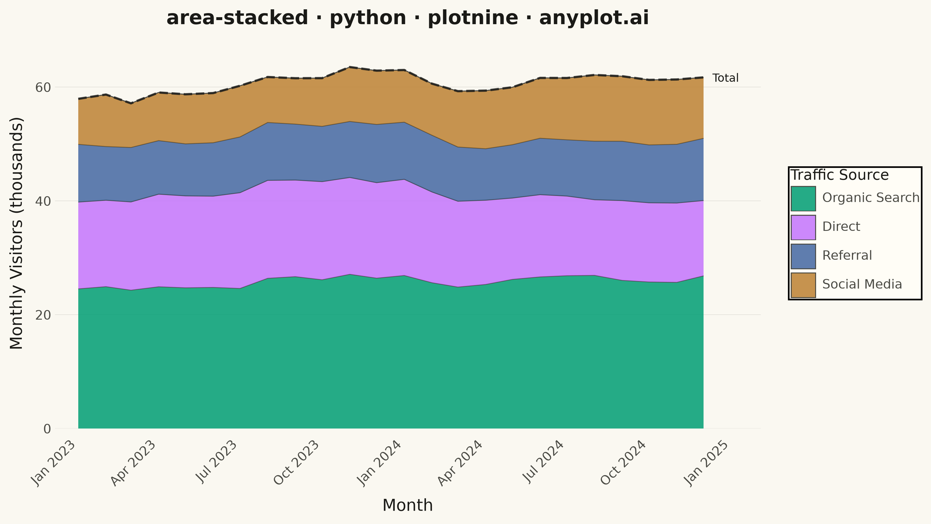
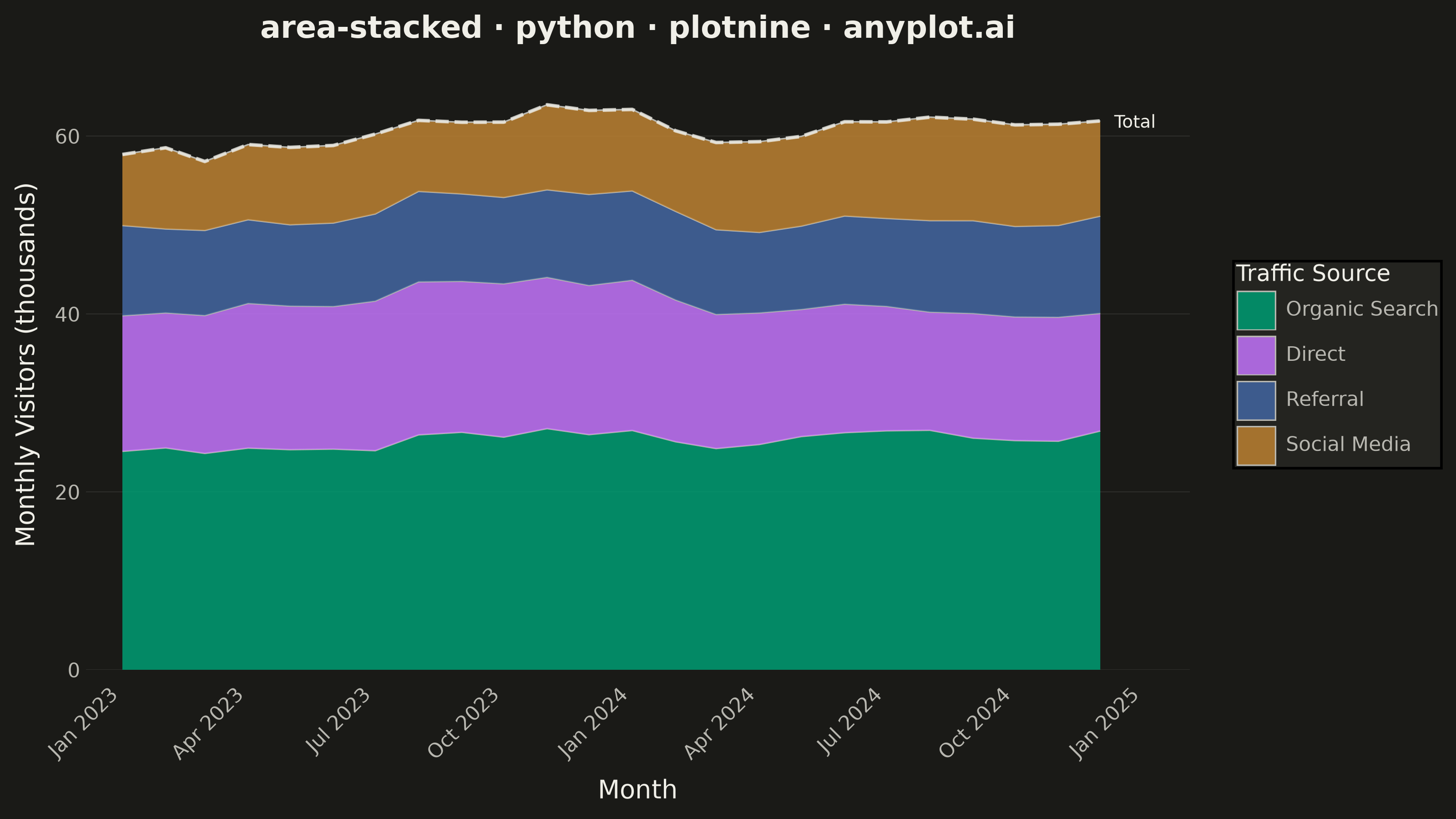
A stacked area chart displays multiple data series as areas stacked on top of each other, with each series starting where the previous one ends. This visualization emphasizes both individual contributions and cumulative totals over a continuous axis (typically time). It is ideal for showing how parts contribute to a whole while tracking changes over time, making patterns of composition and overall trends immediately visible.
""" anyplot.ai
area-stacked: Stacked Area Chart
Library: plotnine 0.15.8 | Python 3.13.15
Quality: 91/100 | Updated: 2026-08-17
"""

import os

import numpy as np
import pandas as pd
from mizani.formatters import comma_format
from plotnine import (
    aes,
    element_blank,
    element_line,
    element_rect,
    element_text,
    geom_area,
    geom_line,
    geom_text,
    ggplot,
    labs,
    position_stack,
    scale_fill_manual,
    scale_x_date,
    scale_y_continuous,
    theme,
    theme_minimal,
)


# Theme tokens
THEME = os.getenv("ANYPLOT_THEME", "light")
PAGE_BG = "#FAF8F1" if THEME == "light" else "#1A1A17"
ELEVATED_BG = "#FFFDF6" if THEME == "light" else "#242420"
INK = "#1A1A17" if THEME == "light" else "#F0EFE8"
INK_SOFT = "#4A4A44" if THEME == "light" else "#B8B7B0"

# Data: website traffic sources over 24 months, in thousands of visitors
np.random.seed(42)

dates = pd.date_range(start="2023-01-01", periods=24, freq="MS")

# Generate realistic traffic data with trends
base_direct = 15000 + np.cumsum(np.random.randn(24) * 500)
base_organic = 25000 + np.cumsum(np.random.randn(24) * 800) + np.arange(24) * 300
base_referral = 10000 + np.cumsum(np.random.randn(24) * 400)
base_social = 8000 + np.cumsum(np.random.randn(24) * 600) + np.arange(24) * 200

# Ensure all values are positive, then rescale to thousands for compact axis labels
direct = np.maximum(base_direct, 5000) / 1000
organic = np.maximum(base_organic, 10000) / 1000
referral = np.maximum(base_referral, 3000) / 1000
social = np.maximum(base_social, 2000) / 1000

# Create long-format DataFrame for stacking
df = pd.DataFrame(
    {
        "Date": np.tile(dates, 4),
        "Visitors": np.concatenate([organic, direct, referral, social]),
        "Source": (["Organic Search"] * 24 + ["Direct"] * 24 + ["Referral"] * 24 + ["Social Media"] * 24),
    }
)

# Order categories by average size (largest at bottom for easier reading)
source_order = ["Organic Search", "Direct", "Referral", "Social Media"]
df["Source"] = pd.Categorical(df["Source"], categories=source_order, ordered=True)

# Running total across sources, overlaid as a dashed trend line so the
# cumulative-traffic story the spec calls out isn't left implicit in the stack
totals = df.groupby("Date", observed=True)["Visitors"].sum().reset_index()
last_total = totals.iloc[[-1]].copy()
last_total["label"] = "Total"

# Imprint palette
colors = ["#009E73", "#C475FD", "#4467A3", "#BD8233"]

# Theme
anyplot_theme = theme(
    figure_size=(8, 4.5),
    plot_background=element_rect(fill=PAGE_BG, color=PAGE_BG),
    panel_background=element_rect(fill=PAGE_BG, color=PAGE_BG),
    panel_grid_major_x=element_blank(),
    panel_grid_major_y=element_line(color=INK, size=0.3, alpha=0.12),
    panel_grid_minor=element_blank(),
    plot_title=element_text(size=12, weight="bold", color=INK),
    axis_title=element_text(size=10, color=INK),
    axis_text=element_text(size=8, color=INK_SOFT),
    axis_text_x=element_text(angle=45, hjust=1, margin={"t": 6, "unit": "pt"}),
    legend_background=element_rect(fill=ELEVATED_BG, color=None),
    legend_text=element_text(size=8, color=INK_SOFT),
    legend_title=element_text(size=9, color=INK),
)

# Create stacked area chart: a subtle ink outline on each band's upper edge
# (outline_type) plus a dashed total-traffic overlay for the cumulative read.
# position_stack(reverse=True) puts the first factor level (Organic Search,
# the largest series) at the bottom of the stack, matching source_order and
# the spec's "largest at bottom" size ordering.
plot = (
    ggplot(df, aes(x="Date", y="Visitors", fill="Source"))
    + geom_area(alpha=0.85, outline_type="upper", color=INK_SOFT, size=0.35, position=position_stack(reverse=True))
    + geom_line(
        totals, aes(x="Date", y="Visitors"), color=INK, linetype="dashed", size=0.8, alpha=0.8, inherit_aes=False
    )
    + geom_text(
        last_total,
        aes(x="Date", y="Visitors", label="label"),
        color=INK,
        size=7,
        ha="left",
        nudge_x=10,
        inherit_aes=False,
    )
    + scale_fill_manual(values=colors)
    + scale_x_date(date_labels="%b %Y", date_breaks="3 months", expand=(0.02, 12, 0.02, 40))
    + scale_y_continuous(labels=comma_format(), expand=(0, 0, 0.08, 0))
    + labs(
        title="area-stacked · python · plotnine · anyplot.ai",
        x="Month",
        y="Monthly Visitors (thousands)",
        fill="Traffic Source",
    )
    + theme_minimal()
    + anyplot_theme
)

# Save
plot.save(f"plot-{THEME}.png", dpi=400, width=8, height=4.5, units="in", verbose=False)
Runnable source as JSON, for any HTTP client: https://api.anyplot.ai/specs/area-stacked/plotnine/code. Any spec id and library id listed in llms-full.txt fit the same URL shape; every URL below is complete and callable.
{
  "spec_id": "area-stacked",
  "language": "python",
  "library": "plotnine",
  "page": "https://anyplot.ai/area-stacked/python/plotnine",
  "hub": "https://anyplot.ai/area-stacked",
  "code_json": "https://api.anyplot.ai/specs/area-stacked/plotnine/code",
  "spec_json": "https://api.anyplot.ai/specs/area-stacked",
  "render_light_png": "https://storage.googleapis.com/anyplot-images/plots/area-stacked/python/plotnine/plot-light.png",
  "render_dark_png": "https://storage.googleapis.com/anyplot-images/plots/area-stacked/python/plotnine/plot-dark.png",
  "quality_score": 91.0,
  "license": "MIT",
  "guide": "https://anyplot.ai/llms.txt"
}
Part of Stacked Area Chart on anyplot.ai.