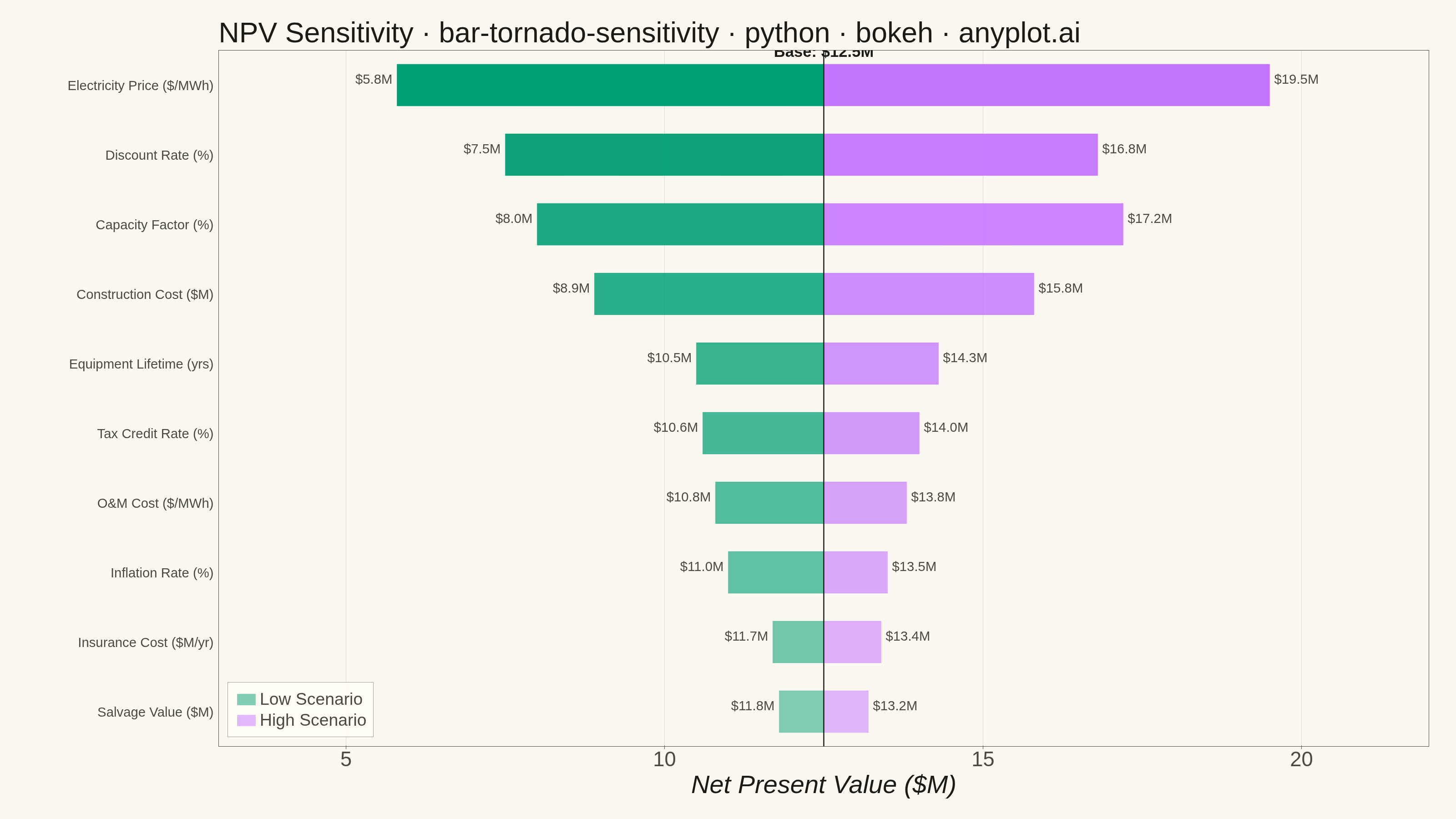
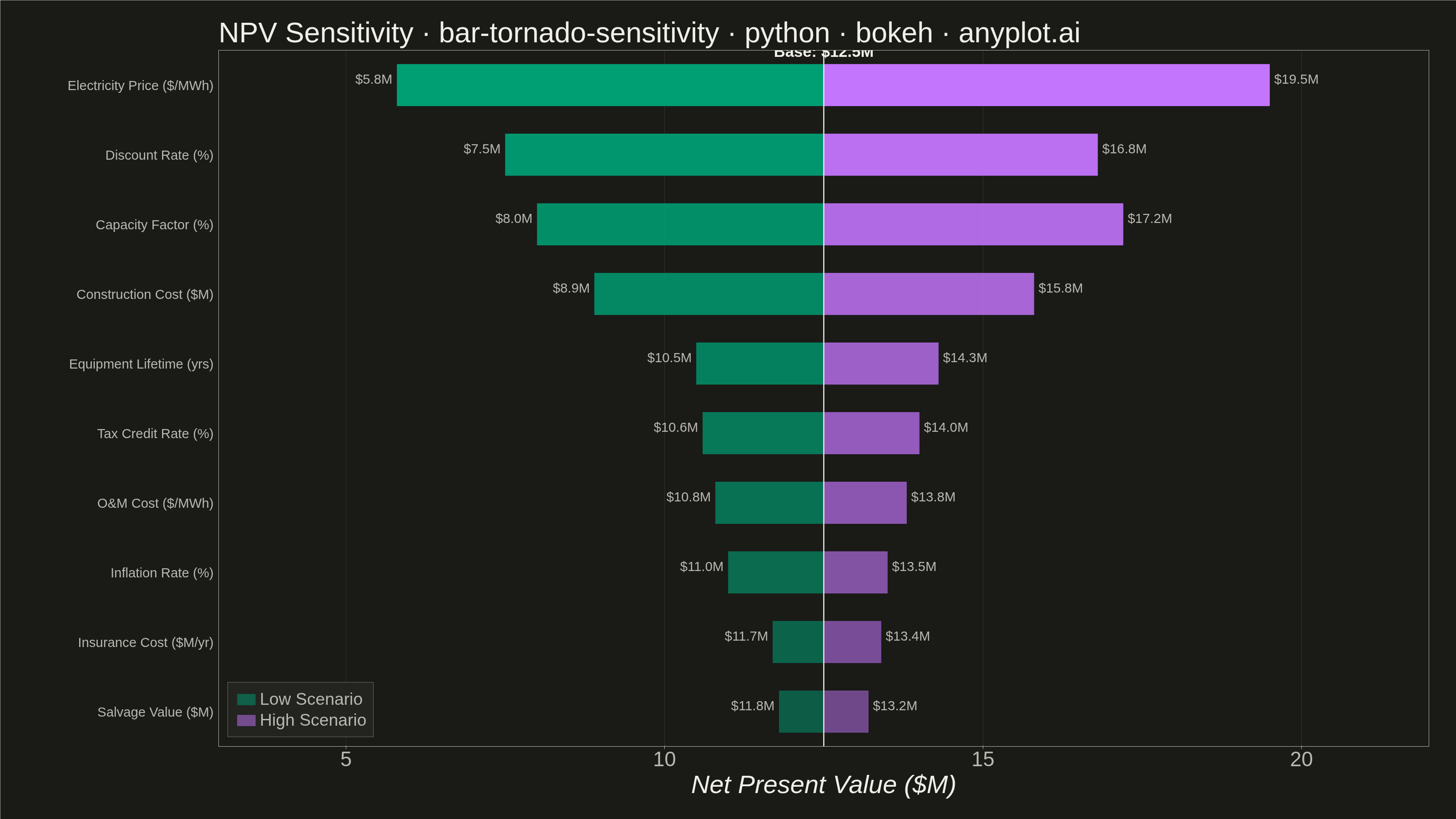
A horizontal bar chart where bars are sorted by influence magnitude, extending left and right from a base case vertical reference line. Each bar represents one input parameter and shows how varying that parameter between its low and high values affects the output, creating a characteristic tornado shape (widest bars at top, narrowest at bottom). Dual colors distinguish low-input from high-input effects, making it immediately clear which parameters drive the most uncertainty.
""" anyplot.ai
bar-tornado-sensitivity: Tornado Diagram for Sensitivity Analysis
Library: bokeh 3.9.0 | Python 3.13.13
Quality: 91/100 | Updated: 2026-06-02
"""

import os
import sys
import time
from pathlib import Path


# Prevent this file (bokeh.py) from shadowing the installed bokeh package
_this_dir = os.path.dirname(os.path.abspath(__file__))
sys.path = [p for p in sys.path if not (p and os.path.abspath(p) == _this_dir)]

import numpy as np
from bokeh.io import output_file, save
from bokeh.models import ColumnDataSource, HoverTool, Label, LabelSet, Span
from bokeh.plotting import figure
from PIL import Image
from selenium import webdriver
from selenium.webdriver.chrome.options import Options


# Theme tokens — Imprint palette
THEME = os.getenv("ANYPLOT_THEME", "light")
PAGE_BG = "#FAF8F1" if THEME == "light" else "#1A1A17"
ELEVATED_BG = "#FFFDF6" if THEME == "light" else "#242420"
INK = "#1A1A17" if THEME == "light" else "#F0EFE8"
INK_SOFT = "#4A4A44" if THEME == "light" else "#B8B7B0"

# Imprint categorical palette — positions 1 and 2 for two series
COLOR_LOW = "#009E73"  # Imprint position 1 — brand green (first series, low scenario)
COLOR_HIGH = "#C475FD"  # Imprint position 2 — lavender (second series, high scenario)

# Data — NPV sensitivity analysis for a renewable energy project
base_npv = 12.5  # Base case NPV ($M)

parameters = [
    "Electricity Price ($/MWh)",
    "Discount Rate (%)",
    "Construction Cost ($M)",
    "Capacity Factor (%)",
    "Equipment Lifetime (yrs)",
    "O&M Cost ($/MWh)",
    "Tax Credit Rate (%)",
    "Inflation Rate (%)",
    "Salvage Value ($M)",
    "Insurance Cost ($M/yr)",
]

# Asymmetric low/high NPV values — more upside on price, more downside on cost
low_values = np.array([5.8, 7.5, 8.9, 8.0, 10.5, 10.8, 10.6, 11.0, 11.8, 11.7])
high_values = np.array([19.5, 16.8, 15.8, 17.2, 14.3, 13.8, 14.0, 13.5, 13.2, 13.4])

# Sort by total range — widest bar at the top of the tornado
total_range = high_values - low_values
sort_idx = np.argsort(total_range)
parameters_sorted = [parameters[i] for i in sort_idx]
low_sorted = low_values[sort_idx]
high_sorted = high_values[sort_idx]
ranges_sorted = total_range[sort_idx]
n = len(parameters_sorted)

# Alpha gradient: more opaque for higher-influence (wider) bars
low_alphas = [0.5 + 0.5 * (i / (n - 1)) for i in range(n)]
high_alphas = [0.5 + 0.5 * (i / (n - 1)) for i in range(n)]

# Bar extents relative to base case
low_left = np.where(low_sorted < base_npv, low_sorted, base_npv)
low_right = np.where(low_sorted < base_npv, base_npv, low_sorted)
high_left = np.where(high_sorted > base_npv, base_npv, high_sorted)
high_right = np.where(high_sorted > base_npv, high_sorted, base_npv)

low_val_fmt = [f"${v:.1f}M" for v in low_sorted]
high_val_fmt = [f"${v:.1f}M" for v in high_sorted]
range_val_fmt = [f"${r:.1f}M" for r in ranges_sorted]

source_low = ColumnDataSource(
    data={
        "parameter": parameters_sorted,
        "left": low_left,
        "right": low_right,
        "low_val": low_val_fmt,
        "high_val": high_val_fmt,
        "range_val": range_val_fmt,
        "alpha": low_alphas,
    }
)

source_high = ColumnDataSource(
    data={
        "parameter": parameters_sorted,
        "left": high_left,
        "right": high_right,
        "low_val": low_val_fmt,
        "high_val": high_val_fmt,
        "range_val": range_val_fmt,
        "alpha": high_alphas,
    }
)

label_low_src = ColumnDataSource(data={"parameter": parameters_sorted, "x": low_sorted, "text": low_val_fmt})

label_high_src = ColumnDataSource(data={"parameter": parameters_sorted, "x": high_sorted, "text": high_val_fmt})

# Title with font scaling for length > 67 chars
title = "NPV Sensitivity · bar-tornado-sensitivity · python · bokeh · anyplot.ai"
title_fontsize = max(34, round(50 * 67 / len(title)))  # 47pt for 71 chars

# Plot — 3200×1800 landscape canvas per hard contract
p = figure(
    width=3200,
    height=1800,
    y_range=parameters_sorted,
    x_range=(3.0, 22.0),
    title=title,
    x_axis_label="Net Present Value ($M)",
    toolbar_location=None,  # prevents toolbar from shrinking canvas height
    min_border_bottom=160,  # room for 34pt x-ticks + 42pt x-axis label
    min_border_left=480,  # extra room for long categorical y-axis labels
    min_border_top=110,  # room for title
    min_border_right=60,
)

# Low-scenario bars
p.hbar(
    y="parameter",
    left="left",
    right="right",
    height=0.6,
    color=COLOR_LOW,
    alpha="alpha",
    source=source_low,
    legend_label="Low Scenario",
    line_color=COLOR_LOW,
    line_width=0.5,
)

# High-scenario bars
p.hbar(
    y="parameter",
    left="left",
    right="right",
    height=0.6,
    color=COLOR_HIGH,
    alpha="alpha",
    source=source_high,
    legend_label="High Scenario",
    line_color=COLOR_HIGH,
    line_width=0.5,
)

# Value annotations at bar ends
low_labels = LabelSet(
    x="x",
    y="parameter",
    text="text",
    source=label_low_src,
    text_font_size="22pt",
    text_color=INK_SOFT,
    text_align="right",
    x_offset=-10,
    y_offset=-3,
)
p.add_layout(low_labels)

high_labels = LabelSet(
    x="x",
    y="parameter",
    text="text",
    source=label_high_src,
    text_font_size="22pt",
    text_color=INK_SOFT,
    text_align="left",
    x_offset=10,
    y_offset=-3,
)
p.add_layout(high_labels)

# Base case vertical reference line
baseline = Span(location=base_npv, dimension="height", line_color=INK, line_width=2.5, line_dash="solid")
p.add_layout(baseline)

# Base case label above top bar
base_label = Label(
    x=base_npv,
    y=n - 0.5,
    text=f"Base: ${base_npv}M",
    text_font_size="26pt",
    text_color=INK,
    text_font_style="bold",
    text_align="center",
    y_units="data",
    y_offset=55,
)
p.add_layout(base_label)

# HoverTool for interactive HTML exploration
hover = HoverTool(
    tooltips=[
        ("Parameter", "@parameter"),
        ("Low NPV", "@low_val"),
        ("High NPV", "@high_val"),
        ("Impact Range", "@range_val"),
    ]
)
p.add_tools(hover)

# Theme-adaptive chrome
p.background_fill_color = PAGE_BG
p.border_fill_color = PAGE_BG
p.outline_line_color = INK_SOFT

p.title.text_font_size = f"{title_fontsize}pt"
p.title.text_color = INK
p.title.text_font_style = "normal"

p.xaxis.axis_label_text_font_size = "42pt"
p.xaxis.axis_label_text_color = INK
p.xaxis.major_label_text_font_size = "34pt"
p.xaxis.major_label_text_color = INK_SOFT
p.xaxis.axis_line_color = INK_SOFT
p.xaxis.major_tick_line_color = INK_SOFT
p.xaxis.minor_tick_line_color = None

p.yaxis.major_label_text_font_size = "22pt"  # smaller for long categorical labels
p.yaxis.major_label_text_color = INK_SOFT
p.yaxis.axis_line_color = None
p.yaxis.major_tick_line_color = None
p.yaxis.minor_tick_line_color = None

p.xgrid.grid_line_color = INK
p.xgrid.grid_line_alpha = 0.12
p.ygrid.grid_line_alpha = 0.0

p.legend.label_text_font_size = "28pt"
p.legend.label_text_color = INK_SOFT
p.legend.background_fill_color = ELEVATED_BG
p.legend.border_line_color = INK_SOFT
p.legend.location = "bottom_left"
p.legend.padding = 15
p.legend.margin = 20
p.legend.glyph_height = 30
p.legend.glyph_width = 50

# Save interactive HTML
output_file(f"plot-{THEME}.html")
save(p)

# Screenshot with headless Chrome — CDP override is authoritative:
# --window-size alone loses ~139 px to Chrome chrome in headless mode
W, H = 3200, 1800
opts = Options()
for arg in (
    "--headless=new",
    "--no-sandbox",
    "--disable-dev-shm-usage",
    "--disable-gpu",
    f"--window-size={W},{H}",
    "--hide-scrollbars",
):
    opts.add_argument(arg)
driver = webdriver.Chrome(options=opts)
driver.execute_cdp_cmd(
    "Emulation.setDeviceMetricsOverride", {"width": W, "height": H, "deviceScaleFactor": 1, "mobile": False}
)
driver.get(f"file://{Path(f'plot-{THEME}.html').resolve()}")
time.sleep(3)
driver.save_screenshot(f"plot-{THEME}.png")
driver.quit()

# PIL safety net: pin to exact 3200×1800 in case of sub-pixel rounding
_img = Image.open(f"plot-{THEME}.png").convert("RGB")
if _img.size != (W, H):
    _norm = Image.new("RGB", (W, H), PAGE_BG)
    _norm.paste(_img, ((W - _img.size[0]) // 2, (H - _img.size[1]) // 2))
    _norm.save(f"plot-{THEME}.png")
Runnable source as JSON, for any HTTP client: https://api.anyplot.ai/specs/bar-tornado-sensitivity/bokeh/code. Any spec id and library id listed in llms-full.txt fit the same URL shape; every URL below is complete and callable.
{
  "spec_id": "bar-tornado-sensitivity",
  "language": "python",
  "library": "bokeh",
  "page": "https://anyplot.ai/bar-tornado-sensitivity/python/bokeh",
  "hub": "https://anyplot.ai/bar-tornado-sensitivity",
  "code_json": "https://api.anyplot.ai/specs/bar-tornado-sensitivity/bokeh/code",
  "spec_json": "https://api.anyplot.ai/specs/bar-tornado-sensitivity",
  "render_light_png": "https://storage.googleapis.com/anyplot-images/plots/bar-tornado-sensitivity/python/bokeh/plot-light.png",
  "render_dark_png": "https://storage.googleapis.com/anyplot-images/plots/bar-tornado-sensitivity/python/bokeh/plot-dark.png",
  "interactive_light_html": "https://storage.googleapis.com/anyplot-images/plots/bar-tornado-sensitivity/python/bokeh/plot-light.html",
  "interactive_dark_html": "https://storage.googleapis.com/anyplot-images/plots/bar-tornado-sensitivity/python/bokeh/plot-dark.html",
  "quality_score": 91.0,
  "license": "MIT",
  "guide": "https://anyplot.ai/llms.txt"
}
Part of Tornado Diagram for Sensitivity Analysis on anyplot.ai.