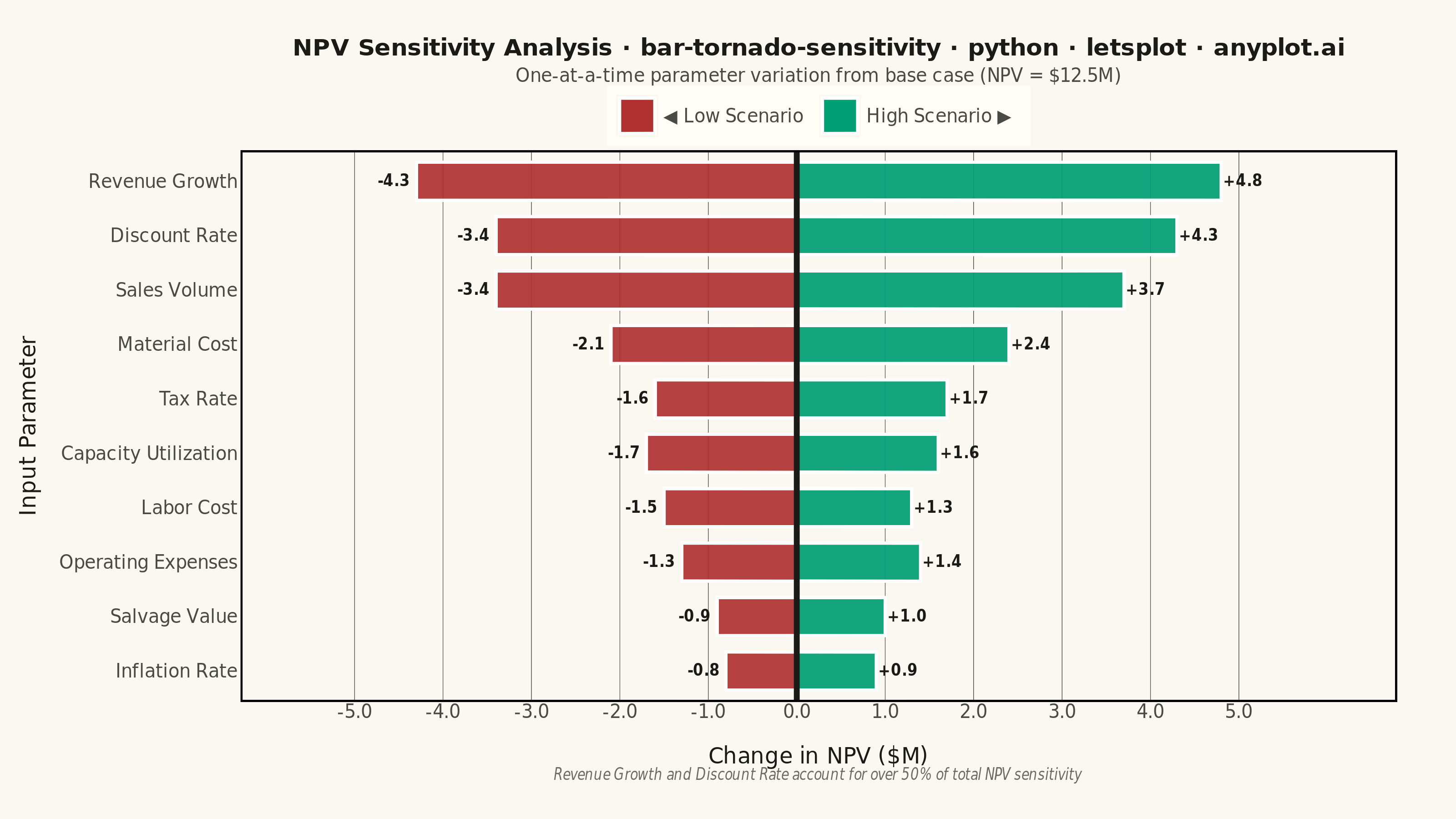
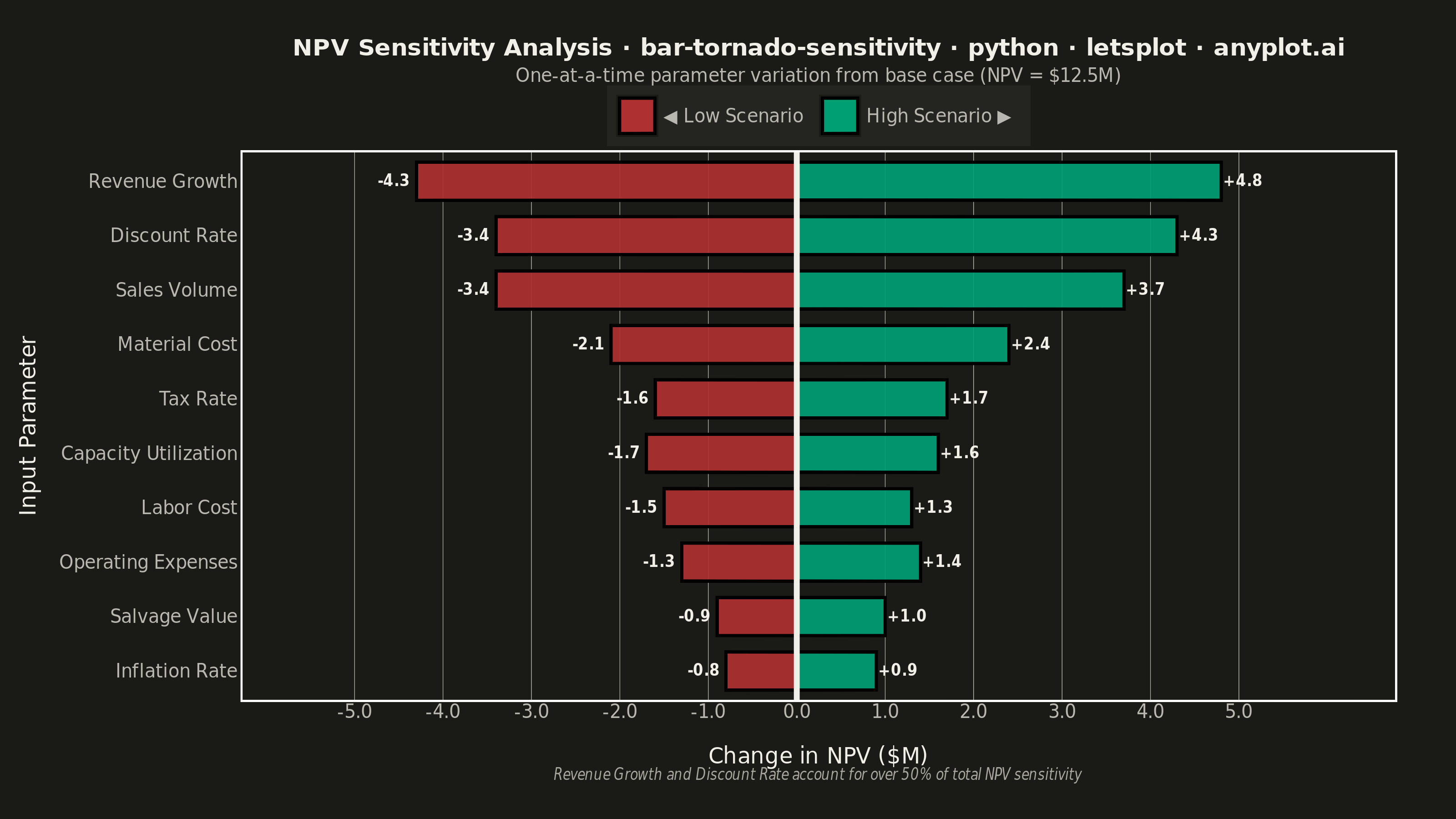
A horizontal bar chart where bars are sorted by influence magnitude, extending left and right from a base case vertical reference line. Each bar represents one input parameter and shows how varying that parameter between its low and high values affects the output, creating a characteristic tornado shape (widest bars at top, narrowest at bottom). Dual colors distinguish low-input from high-input effects, making it immediately clear which parameters drive the most uncertainty.
""" anyplot.ai
bar-tornado-sensitivity: Tornado Diagram for Sensitivity Analysis
Library: letsplot 4.10.1 | Python 3.13.13
Quality: 90/100 | Updated: 2026-06-02
"""

import os

import pandas as pd
from lets_plot import (
    LetsPlot,
    aes,
    element_blank,
    element_line,
    element_rect,
    element_text,
    flavor_high_contrast_dark,
    flavor_high_contrast_light,
    geom_bar,
    geom_text,
    geom_vline,
    ggplot,
    ggsave,
    ggsize,
    labs,
    layer_tooltips,
    scale_fill_manual,
    scale_x_continuous,
    theme,
    theme_minimal,
)


LetsPlot.setup_html()

# Theme tokens — Imprint palette, theme-adaptive chrome
THEME = os.getenv("ANYPLOT_THEME", "light")
PAGE_BG = "#FAF8F1" if THEME == "light" else "#1A1A17"
ELEVATED_BG = "#FFFDF6" if THEME == "light" else "#242420"
INK = "#1A1A17" if THEME == "light" else "#F0EFE8"
INK_SOFT = "#4A4A44" if THEME == "light" else "#B8B7B0"
INK_MUTED = "#6B6A63" if THEME == "light" else "#A8A79F"

# Imprint palette — semantic exception: gain/loss for financial sensitivity
# High Scenario (upper NPV bound) → #009E73 brand green (profit/gain)
# Low Scenario  (lower NPV bound) → #AE3030 matte red  (loss/downside)
COLOR_HIGH = "#009E73"
COLOR_LOW = "#AE3030"

# Data — NPV sensitivity analysis for a capital investment project
base_npv = 12.5  # Base case NPV in $M

parameters = [
    "Discount Rate",
    "Revenue Growth",
    "Material Cost",
    "Labor Cost",
    "Sales Volume",
    "Tax Rate",
    "Salvage Value",
    "Operating Expenses",
    "Inflation Rate",
    "Capacity Utilization",
]

low_values = [16.8, 8.2, 14.9, 13.8, 9.1, 14.2, 11.6, 13.9, 13.4, 10.8]
high_values = [9.1, 17.3, 10.4, 11.0, 16.2, 10.9, 13.5, 11.2, 11.7, 14.1]

df = pd.DataFrame({"parameter": parameters, "low_value": low_values, "high_value": high_values})

# Sort by total range (widest bar at top)
df["total_range"] = abs(df["high_value"] - df["low_value"])
df = df.sort_values("total_range", ascending=True).reset_index(drop=True)

# Build long-form data: each parameter gets two bars (low side and high side)
rows = []
for _, row in df.iterrows():
    low_side = min(row["low_value"], row["high_value"])
    high_side = max(row["low_value"], row["high_value"])
    low_delta = low_side - base_npv
    high_delta = high_side - base_npv

    low_nudge = low_delta - 0.25
    high_nudge = high_delta + 0.25

    rows.append(
        {
            "parameter": row["parameter"],
            "value": low_delta,
            "scenario": "Low Scenario",
            "label": f"{low_delta:+.1f}",
            "npv": f"${low_side:.1f}M",
            "label_x": low_nudge,
        }
    )
    rows.append(
        {
            "parameter": row["parameter"],
            "value": high_delta,
            "scenario": "High Scenario",
            "label": f"{high_delta:+.1f}",
            "npv": f"${high_side:.1f}M",
            "label_x": high_nudge,
        }
    )

plot_df = pd.DataFrame(rows)

# Preserve sorted order (ascending range = narrowest at bottom, widest at top)
param_order = df["parameter"].tolist()
plot_df["parameter"] = pd.Categorical(plot_df["parameter"], categories=param_order, ordered=True)

# Title — scale fontsize for 83-char title (default 16, floor 11)
TITLE = "NPV Sensitivity Analysis · bar-tornado-sensitivity · python · letsplot · anyplot.ai"
title_fs = max(11, round(16 * 67 / len(TITLE)))

flavor = flavor_high_contrast_light() if THEME == "light" else flavor_high_contrast_dark()

# Plot
plot = (
    ggplot(plot_df, aes(x="value", y="parameter", fill="scenario"))
    + geom_bar(
        stat="identity",
        width=0.7,
        alpha=0.92,
        position="identity",
        tooltips=layer_tooltips()
        .line("@parameter")
        .line("Scenario: @scenario")
        .line("NPV Impact: @label $M")
        .line("Resulting NPV: @npv"),
    )
    + geom_vline(xintercept=0, color=INK, size=1.4, linetype="solid")
    + geom_text(
        aes(x="label_x", label="label"),
        position="identity",
        hjust=1.1,
        size=4,
        color=INK,
        fontface="bold",
        data=plot_df[plot_df["scenario"] == "Low Scenario"],
    )
    + geom_text(
        aes(x="label_x", label="label"),
        position="identity",
        hjust=-0.1,
        size=4,
        color=INK,
        fontface="bold",
        data=plot_df[plot_df["scenario"] == "High Scenario"],
    )
    + scale_fill_manual(
        values=[COLOR_LOW, COLOR_HIGH],
        breaks=["Low Scenario", "High Scenario"],
        labels=["◀ Low Scenario", "High Scenario ▶"],
    )
    + scale_x_continuous(expand=[0.18, 0], format="{.1f}", breaks=[-5, -4, -3, -2, -1, 0, 1, 2, 3, 4, 5])
    + labs(
        x="Change in NPV ($M)",
        y="Input Parameter",
        title=TITLE,
        subtitle="One-at-a-time parameter variation from base case (NPV = $12.5M)",
        caption="Revenue Growth and Discount Rate account for over 50% of total NPV sensitivity",
        fill="",
    )
    + theme_minimal()
    + flavor
    + theme(
        plot_background=element_rect(fill=PAGE_BG, color=PAGE_BG),
        panel_background=element_rect(fill=PAGE_BG),
        plot_title=element_text(size=title_fs, face="bold", hjust=0.5, color=INK),
        plot_subtitle=element_text(size=10, hjust=0.5, color=INK_SOFT),
        axis_title_x=element_text(size=12, margin=[10, 0, 0, 0], color=INK),
        axis_title_y=element_text(size=12, color=INK),
        axis_text_x=element_text(size=10, color=INK_SOFT),
        axis_text_y=element_text(size=10, color=INK_SOFT),
        legend_text=element_text(size=10, color=INK_SOFT),
        legend_title=element_blank(),
        legend_position="top",
        legend_background=element_rect(fill=ELEVATED_BG, color=INK_SOFT),
        panel_grid_major_y=element_blank(),
        panel_grid_minor=element_blank(),
        panel_grid_major_x=element_line(color=INK_SOFT, size=0.3),
        plot_caption=element_text(size=8, color=INK_MUTED, face="italic", hjust=0.5),
        plot_margin=[20, 30, 20, 10],
    )
    + ggsize(800, 450)  # 800 × 450 × scale=4 = 3200 × 1800 px (landscape)
)

# Save
ggsave(plot, f"plot-{THEME}.png", path=".", scale=4)
ggsave(plot, f"plot-{THEME}.html", path=".")
Runnable source as JSON, for any HTTP client: https://api.anyplot.ai/specs/bar-tornado-sensitivity/letsplot/code. Any spec id and library id listed in llms-full.txt fit the same URL shape; every URL below is complete and callable.
{
  "spec_id": "bar-tornado-sensitivity",
  "language": "python",
  "library": "letsplot",
  "page": "https://anyplot.ai/bar-tornado-sensitivity/python/letsplot",
  "hub": "https://anyplot.ai/bar-tornado-sensitivity",
  "code_json": "https://api.anyplot.ai/specs/bar-tornado-sensitivity/letsplot/code",
  "spec_json": "https://api.anyplot.ai/specs/bar-tornado-sensitivity",
  "render_light_png": "https://storage.googleapis.com/anyplot-images/plots/bar-tornado-sensitivity/python/letsplot/plot-light.png",
  "render_dark_png": "https://storage.googleapis.com/anyplot-images/plots/bar-tornado-sensitivity/python/letsplot/plot-dark.png",
  "interactive_light_html": "https://storage.googleapis.com/anyplot-images/plots/bar-tornado-sensitivity/python/letsplot/plot-light.html",
  "interactive_dark_html": "https://storage.googleapis.com/anyplot-images/plots/bar-tornado-sensitivity/python/letsplot/plot-dark.html",
  "quality_score": 90.0,
  "license": "MIT",
  "guide": "https://anyplot.ai/llms.txt"
}
Part of Tornado Diagram for Sensitivity Analysis on anyplot.ai.