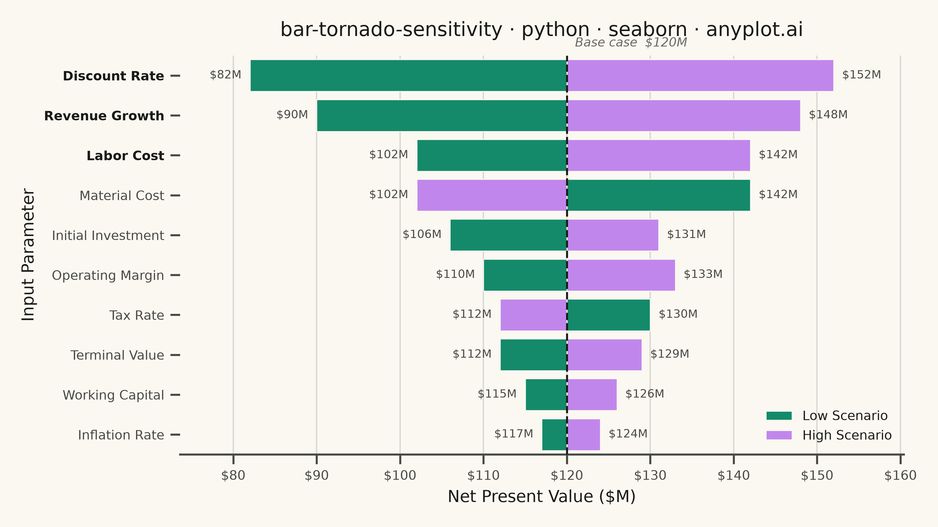
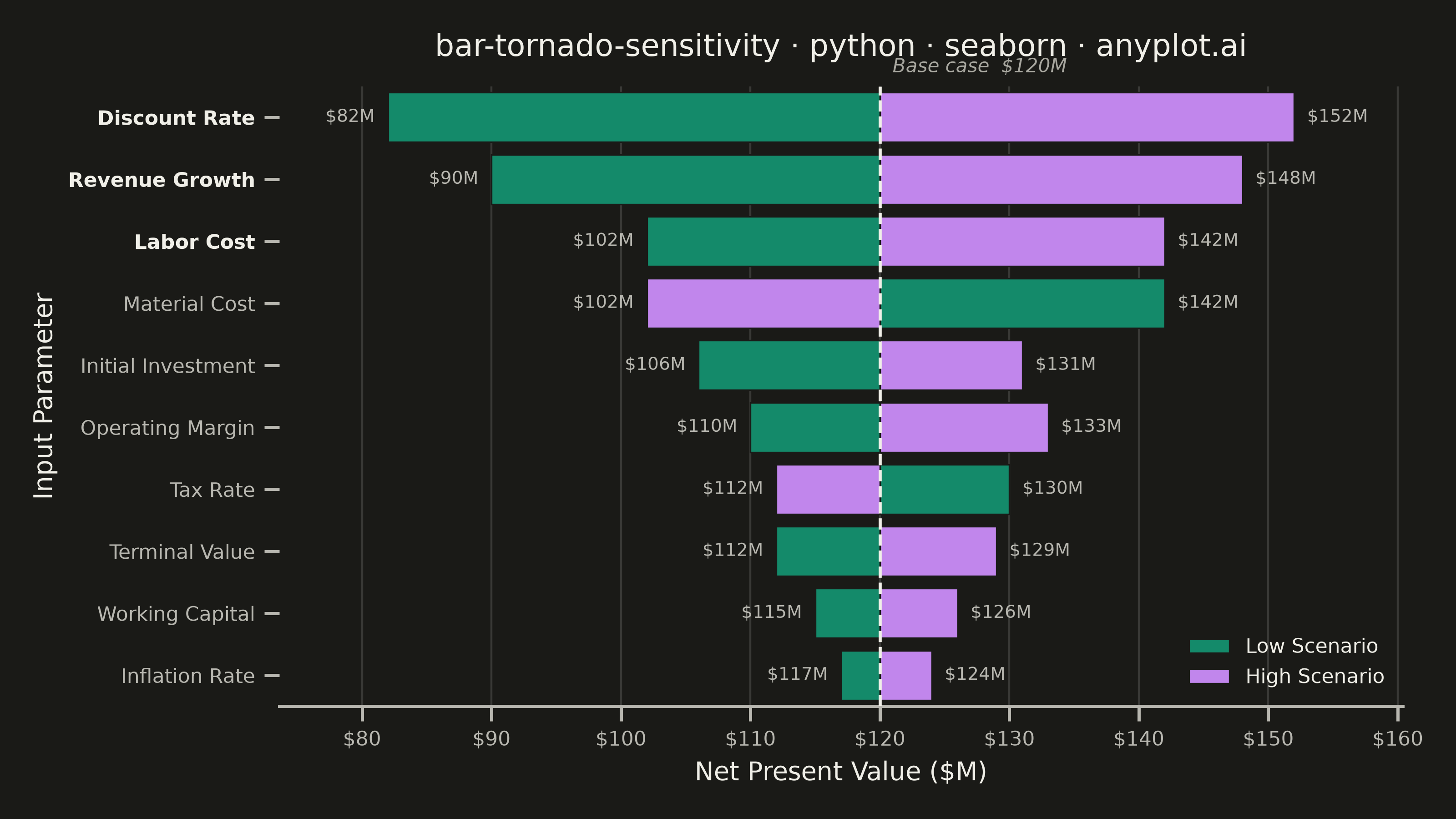
A horizontal bar chart where bars are sorted by influence magnitude, extending left and right from a base case vertical reference line. Each bar represents one input parameter and shows how varying that parameter between its low and high values affects the output, creating a characteristic tornado shape (widest bars at top, narrowest at bottom). Dual colors distinguish low-input from high-input effects, making it immediately clear which parameters drive the most uncertainty.
""" anyplot.ai
bar-tornado-sensitivity: Tornado Diagram for Sensitivity Analysis
Library: seaborn 0.13.2 | Python 3.13.13
Quality: 90/100 | Updated: 2026-06-16
"""

import os

import matplotlib.pyplot as plt
import numpy as np
import pandas as pd
import seaborn as sns


# Theme tokens (see prompts/default-style-guide.md "Theme-adaptive Chrome")
THEME = os.getenv("ANYPLOT_THEME", "light")
PAGE_BG = "#FAF8F1" if THEME == "light" else "#1A1A17"
ELEVATED_BG = "#FFFDF6" if THEME == "light" else "#242420"
INK = "#1A1A17" if THEME == "light" else "#F0EFE8"
INK_SOFT = "#4A4A44" if THEME == "light" else "#B8B7B0"
INK_MUTED = "#6B6A63" if THEME == "light" else "#A8A79F"

# Imprint palette — first categorical series is ALWAYS brand green
BRAND = "#009E73"  # Low Scenario
LAVENDER = "#C475FD"  # High Scenario (Imprint position 2)

sns.set_theme(
    style="ticks",
    rc={
        "figure.facecolor": PAGE_BG,
        "axes.facecolor": PAGE_BG,
        "axes.edgecolor": INK_SOFT,
        "axes.labelcolor": INK,
        "text.color": INK,
        "xtick.color": INK_SOFT,
        "ytick.color": INK_SOFT,
        "grid.color": INK,
        "grid.alpha": 0.15,
        "legend.facecolor": ELEVATED_BG,
        "legend.edgecolor": INK_SOFT,
    },
)

# Data — NPV sensitivity analysis for a capital investment project
parameters = [
    "Discount Rate",
    "Revenue Growth",
    "Material Cost",
    "Labor Cost",
    "Tax Rate",
    "Initial Investment",
    "Operating Margin",
    "Terminal Value",
    "Working Capital",
    "Inflation Rate",
]

base_npv = 120.0  # Base case NPV in $M

# Resulting NPV when each parameter is set to its low / high value.
# Some parameters invert (lower material cost or tax rate → higher NPV).
low_values = base_npv + np.array([-38, -30, 22, -18, 10, -14, -10, -8, -5, -3], dtype=float)
high_values = base_npv + np.array([32, 28, -18, 22, -8, 11, 13, 9, 6, 4], dtype=float)

# Sort by total impact range so the widest bar lands at the top (tornado shape).
# Seaborn draws the first category at the top row, so order widest-first.
total_range = np.abs(high_values - low_values)
sort_idx = np.argsort(total_range)[::-1]
parameters = [parameters[i] for i in sort_idx]
low_values = low_values[sort_idx]
high_values = high_values[sort_idx]

# Deltas relative to the base case (bars diverge from the reference line)
low_delta = low_values - base_npv
high_delta = high_values - base_npv

# Long-form DataFrame for seaborn's hue API
df = pd.concat(
    [
        pd.DataFrame({"Parameter": parameters, "Delta": low_delta, "Scenario": "Low Scenario"}),
        pd.DataFrame({"Parameter": parameters, "Delta": high_delta, "Scenario": "High Scenario"}),
    ],
    ignore_index=True,
)

# Plot — landscape 3200×1800
fig, ax = plt.subplots(figsize=(8, 4.5), dpi=400, facecolor=PAGE_BG)
ax.set_facecolor(PAGE_BG)

sns.barplot(
    data=df,
    y="Parameter",
    x="Delta",
    hue="Scenario",
    hue_order=["Low Scenario", "High Scenario"],
    palette=[BRAND, LAVENDER],
    dodge=False,
    edgecolor=PAGE_BG,
    linewidth=0.6,
    zorder=2,
    ax=ax,
)

# Base case reference line (neutral / baseline anchor)
ax.axvline(x=0, color=INK, linewidth=1.2, linestyle="--", zorder=3)
ax.annotate(
    f"Base case  ${int(base_npv)}M",
    xy=(0, 0),
    xytext=(5, 16),
    textcoords="offset points",
    fontsize=7.5,
    fontstyle="italic",
    color=INK_MUTED,
    ha="left",
    va="bottom",
    annotation_clip=False,
)

# Bar-end value labels — resulting NPV at each scenario end
for i in range(len(parameters)):
    ld, hd = low_delta[i], high_delta[i]
    lv, hv = low_values[i], high_values[i]
    left_x, right_x = min(ld, hd), max(ld, hd)
    left_v, right_v = (lv, hv) if ld <= hd else (hv, lv)
    ax.text(left_x - 1.0, i, f"${left_v:.0f}M", va="center", ha="right", fontsize=7, color=INK_SOFT)
    ax.text(right_x + 1.0, i, f"${right_v:.0f}M", va="center", ha="left", fontsize=7, color=INK_SOFT)

# Relabel x ticks to absolute NPV values
ticks = ax.get_xticks()
ax.set_xticks(ticks)
ax.set_xticklabels([f"${int(t + base_npv)}" for t in ticks])

# Emphasize the three most impactful parameters (widest bars, at the top)
for i, label in enumerate(ax.get_yticklabels()):
    if i < 3:
        label.set_fontweight("bold")
        label.set_color(INK)

# Style
ax.set_xlabel("Net Present Value ($M)", fontsize=10, color=INK)
ax.set_ylabel("Input Parameter", fontsize=10, color=INK)
ax.set_title(
    "bar-tornado-sensitivity · python · seaborn · anyplot.ai", fontsize=12, fontweight="medium", color=INK, pad=12
)
ax.tick_params(axis="both", labelsize=8)
ax.margins(x=0.12)

sns.despine(left=True, bottom=False, ax=ax)
ax.yaxis.grid(False)
ax.xaxis.grid(True, alpha=0.15, linewidth=0.8, color=INK)
ax.set_axisbelow(True)

ax.legend(fontsize=8, frameon=False, loc="lower right")

fig.tight_layout()
plt.savefig(f"plot-{THEME}.png", dpi=400, facecolor=PAGE_BG)
Runnable source as JSON, for any HTTP client: https://api.anyplot.ai/specs/bar-tornado-sensitivity/seaborn/code. Any spec id and library id listed in llms-full.txt fit the same URL shape; every URL below is complete and callable.
{
  "spec_id": "bar-tornado-sensitivity",
  "language": "python",
  "library": "seaborn",
  "page": "https://anyplot.ai/bar-tornado-sensitivity/python/seaborn",
  "hub": "https://anyplot.ai/bar-tornado-sensitivity",
  "code_json": "https://api.anyplot.ai/specs/bar-tornado-sensitivity/seaborn/code",
  "spec_json": "https://api.anyplot.ai/specs/bar-tornado-sensitivity",
  "render_light_png": "https://storage.googleapis.com/anyplot-images/plots/bar-tornado-sensitivity/python/seaborn/plot-light.png",
  "render_dark_png": "https://storage.googleapis.com/anyplot-images/plots/bar-tornado-sensitivity/python/seaborn/plot-dark.png",
  "quality_score": 90.0,
  "license": "MIT",
  "guide": "https://anyplot.ai/llms.txt"
}
Part of Tornado Diagram for Sensitivity Analysis on anyplot.ai.