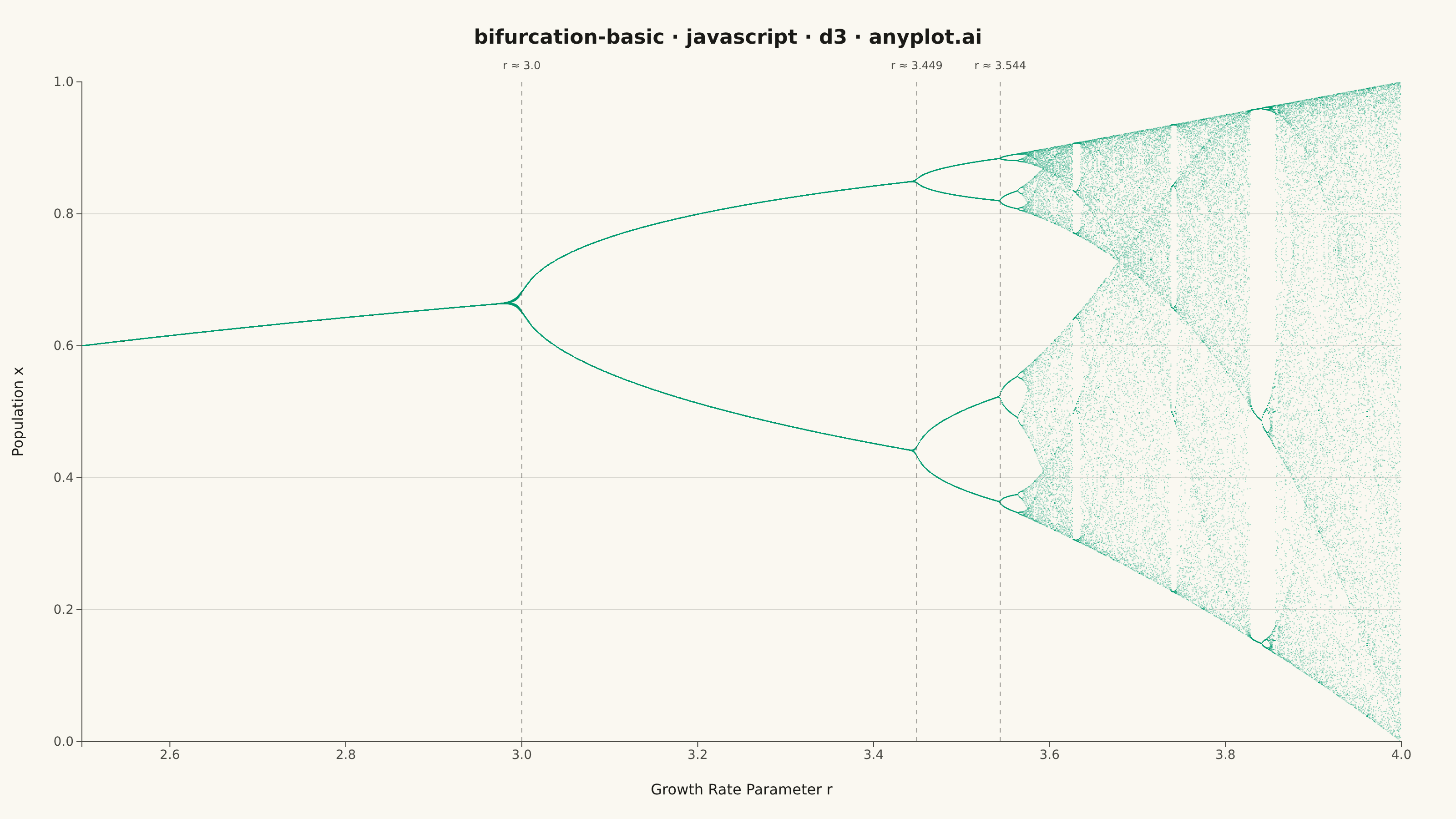
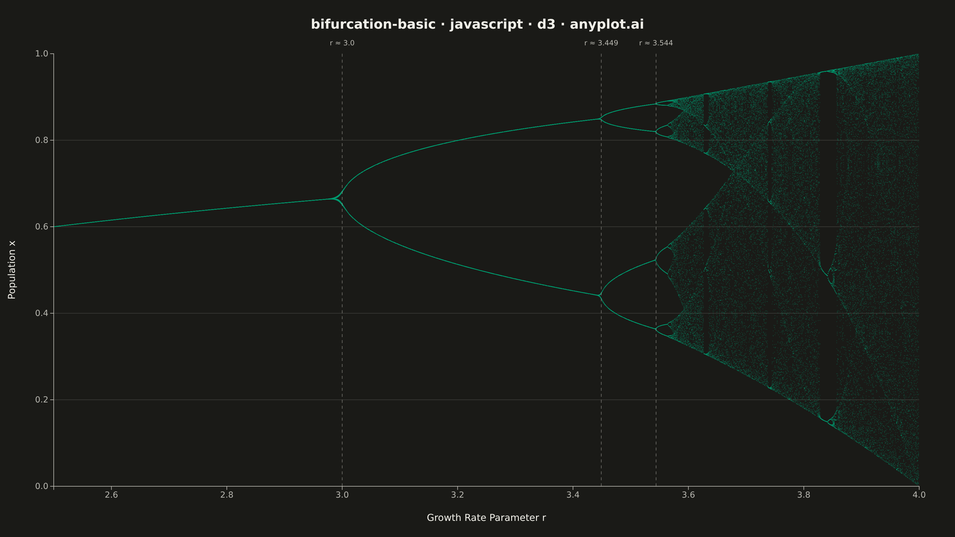
Bifurcation Diagram for Dynamical Systems — D3.js

A bifurcation diagram shows how the steady-state behavior of a dynamical system changes as a control parameter varies. By plotting the long-term values of a state variable against a continuously varied parameter, it reveals transitions from stable fixed points through period-doubling cascades to chaotic regimes. The classic example is the logistic map, where the route to chaos is clearly visible as the growth rate parameter increases.

Bifurcation Diagram for Dynamical Systems rendered with D3.js

JavaScript source (D3.js)

// anyplot.ai
// bifurcation-basic: Bifurcation Diagram for Dynamical Systems
// Library: d3 7.9.0 | JavaScript 22.22.3
// Quality: 91/100 | Created: 2026-06-17

const t = window.ANYPLOT_TOKENS;
const { width, height } = window.ANYPLOT_SIZE;

const margin = { top: 90, right: 60, bottom: 85, left: 90 };
const iw = width - margin.left - margin.right;
const ih = height - margin.top - margin.bottom;

// Container layout — canvas + SVG stack
const container = document.getElementById('container');
container.style.position = 'relative';
container.style.overflow = 'hidden';

// Canvas for data points (2× DPR so pixels are crisp at deviceScaleFactor 2)
const DPR = 2;
const canvas = document.createElement('canvas');
canvas.width = width * DPR;
canvas.height = height * DPR;
canvas.style.width = width + 'px';
canvas.style.height = height + 'px';
canvas.style.position = 'absolute';
canvas.style.top = '0';
canvas.style.left = '0';
container.appendChild(canvas);

const ctx = canvas.getContext('2d');
ctx.scale(DPR, DPR);

// Background
ctx.fillStyle = t.pageBg;
ctx.fillRect(0, 0, width, height);

// D3 scales
const rMin = 2.5, rMax = 4.0;
const xScale = d3.scaleLinear().domain([rMin, rMax]).range([margin.left, margin.left + iw]);
const yScale = d3.scaleLinear().domain([0, 1]).range([margin.top + ih, margin.top]);

// Horizontal gridlines drawn before data so they sit behind the points
const yGridVals = [0.2, 0.4, 0.6, 0.8];
ctx.strokeStyle = t.grid;
ctx.lineWidth = 1;
yGridVals.forEach(v => {
  const cy = yScale(v);
  ctx.beginPath();
  ctx.moveTo(margin.left, cy);
  ctx.lineTo(margin.left + iw, cy);
  ctx.stroke();
});

// Clip to chart area then draw bifurcation data
ctx.save();
ctx.beginPath();
ctx.rect(margin.left, margin.top, iw, ih);
ctx.clip();

const numR = 1500;
const transient = 200;
const plotIter = 100;

ctx.globalAlpha = 0.38;
ctx.fillStyle = t.palette[0]; // #009E73 — Imprint brand green, always first series

for (let i = 0; i <= numR; i++) {
  const r = rMin + (rMax - rMin) * i / numR;
  let x = 0.5;
  for (let j = 0; j < transient; j++) {
    x = r * x * (1 - x);
  }
  const cx = xScale(r);
  for (let j = 0; j < plotIter; j++) {
    x = r * x * (1 - x);
    const cy = yScale(x);
    ctx.fillRect(cx - 0.5, cy - 0.5, 1, 1);
  }
}

ctx.restore();

// SVG overlay — axes, labels, bifurcation markers, title
const svg = d3.select('#container').append('svg')
  .attr('width', width)
  .attr('height', height)
  .style('position', 'absolute')
  .style('top', '0')
  .style('left', '0');

// X axis
const xAxisG = svg.append('g')
  .attr('transform', `translate(0,${margin.top + ih})`)
  .call(d3.axisBottom(xScale).ticks(7).tickFormat(d3.format('.1f')));

xAxisG.selectAll('text')
  .attr('fill', t.inkSoft)
  .style('font-size', '14px')
  .style('font-family', 'system-ui, sans-serif');
xAxisG.selectAll('.tick line').attr('stroke', t.inkSoft);
xAxisG.select('.domain').attr('stroke', t.inkSoft);

// Y axis
const yAxisG = svg.append('g')
  .attr('transform', `translate(${margin.left},0)`)
  .call(d3.axisLeft(yScale).ticks(5).tickFormat(d3.format('.1f')));

yAxisG.selectAll('text')
  .attr('fill', t.inkSoft)
  .style('font-size', '14px')
  .style('font-family', 'system-ui, sans-serif');
yAxisG.selectAll('.tick line').attr('stroke', t.inkSoft);
yAxisG.select('.domain').attr('stroke', t.inkSoft);

// Bifurcation point markers (dashed verticals + labels above chart)
const bifPoints = [
  { r: 3.0, label: 'r ≈ 3.0' },
  { r: 3.449, label: 'r ≈ 3.449' },
  { r: 3.544, label: 'r ≈ 3.544' },
];

bifPoints.forEach(({ r, label }) => {
  const cx = xScale(r);

  svg.append('line')
    .attr('x1', cx).attr('x2', cx)
    .attr('y1', margin.top).attr('y2', margin.top + ih)
    .attr('stroke', t.inkSoft)
    .attr('stroke-width', 1)
    .attr('stroke-dasharray', '5,5')
    .attr('opacity', 0.55);

  svg.append('text')
    .attr('x', cx)
    .attr('y', margin.top - 14)
    .attr('text-anchor', 'middle')
    .attr('fill', t.inkSoft)
    .style('font-size', '12px')
    .style('font-family', 'system-ui, sans-serif')
    .text(label);
});

// Axis labels
svg.append('text')
  .attr('x', margin.left + iw / 2)
  .attr('y', margin.top + ih + 58)
  .attr('text-anchor', 'middle')
  .attr('fill', t.ink)
  .style('font-size', '16px')
  .style('font-family', 'system-ui, sans-serif')
  .text('Growth Rate Parameter r');

svg.append('text')
  .attr('transform', `translate(${margin.left - 65},${margin.top + ih / 2}) rotate(-90)`)
  .attr('text-anchor', 'middle')
  .attr('fill', t.ink)
  .style('font-size', '16px')
  .style('font-family', 'system-ui, sans-serif')
  .text('Population x');

// Title
svg.append('text')
  .attr('x', width / 2)
  .attr('y', 48)
  .attr('text-anchor', 'middle')
  .attr('fill', t.ink)
  .style('font-size', '22px')
  .style('font-weight', '600')
  .style('font-family', 'system-ui, sans-serif')
  .text('bifurcation-basic · javascript · d3 · anyplot.ai');

Part of Bifurcation Diagram for Dynamical Systems on anyplot.ai.

Bifurcation Diagram for Dynamical Systems — D3.js

JavaScript source (D3.js)

Other implementations