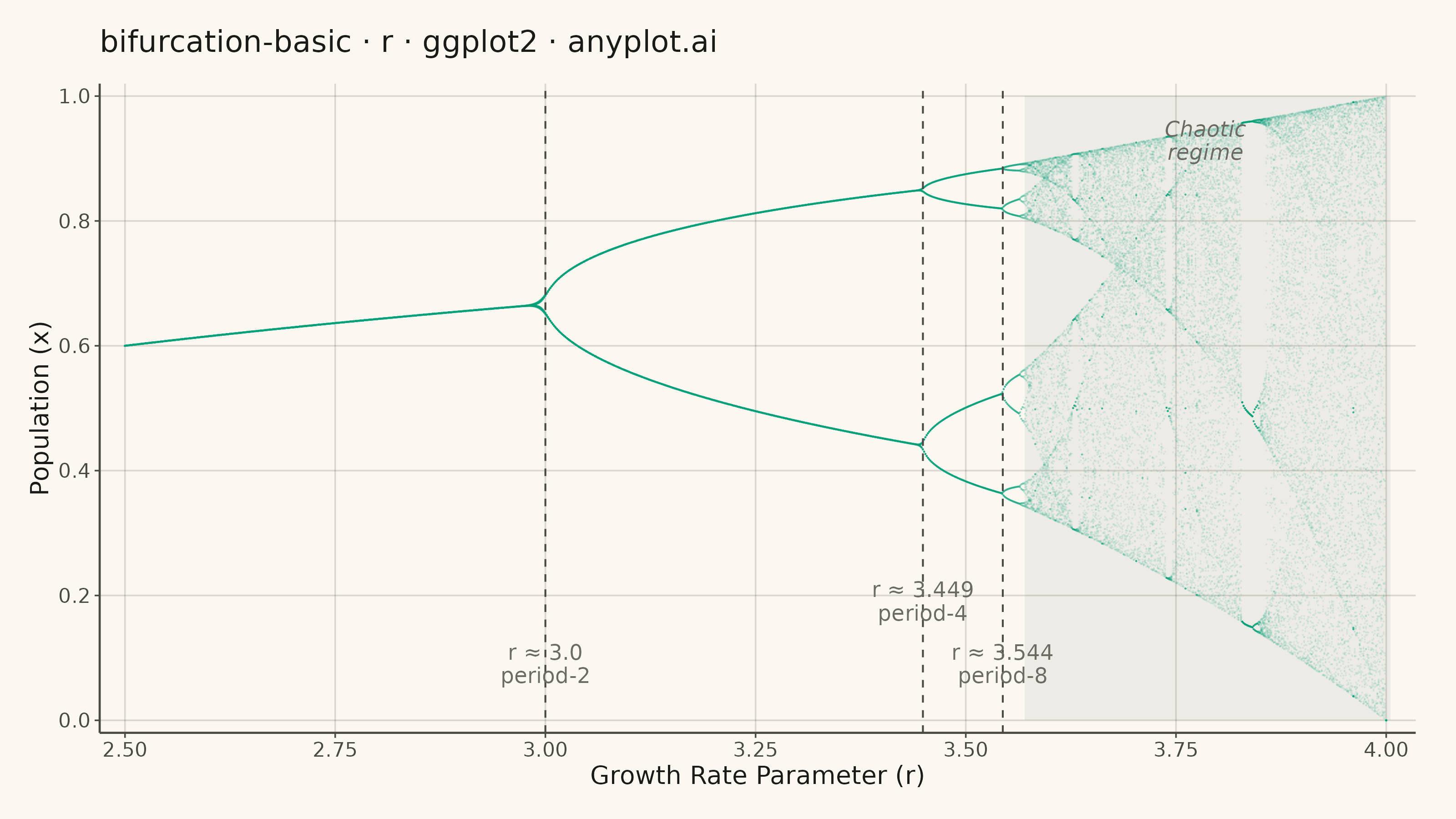
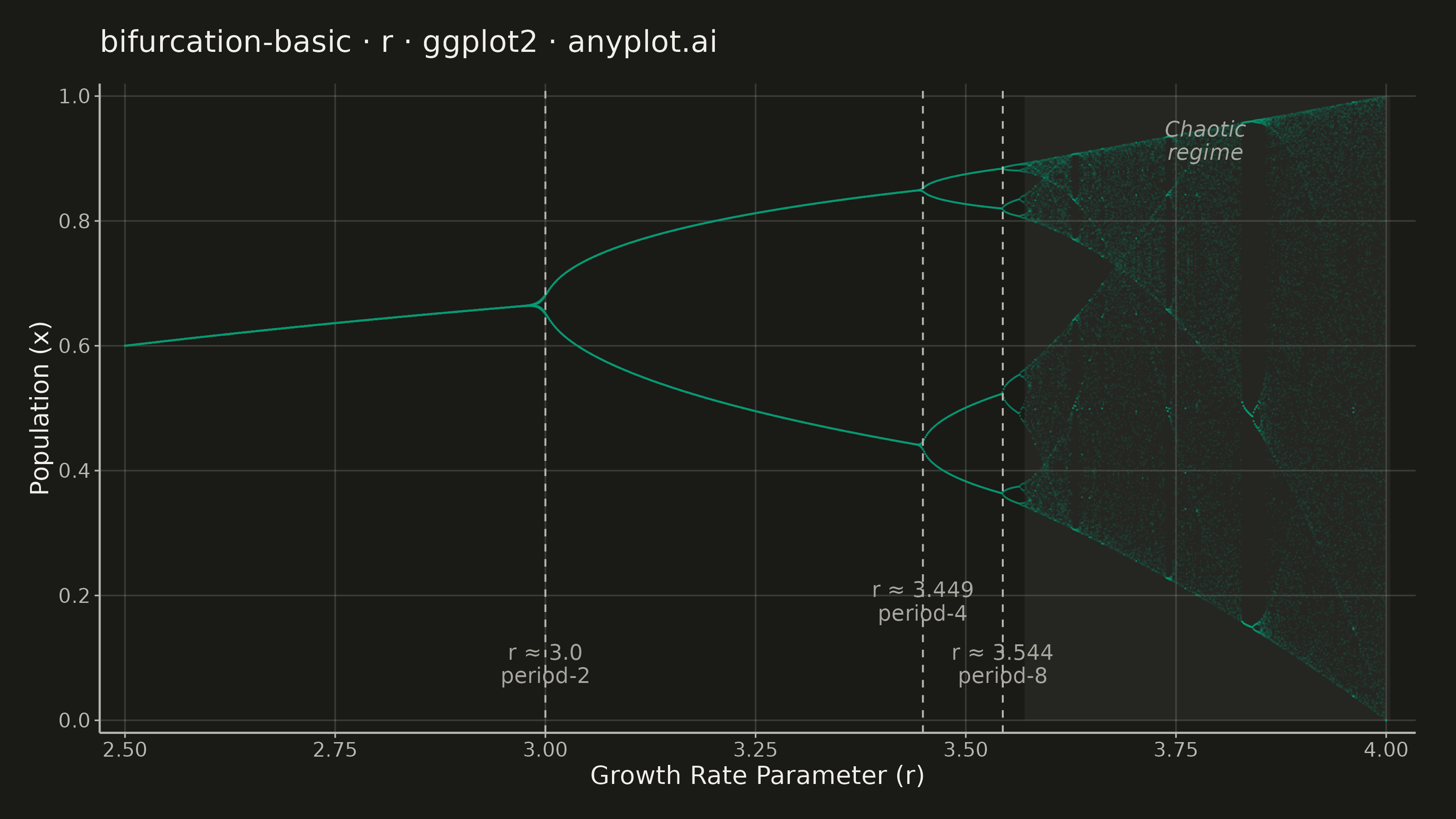
A bifurcation diagram shows how the steady-state behavior of a dynamical system changes as a control parameter varies. By plotting the long-term values of a state variable against a continuously varied parameter, it reveals transitions from stable fixed points through period-doubling cascades to chaotic regimes. The classic example is the logistic map, where the route to chaos is clearly visible as the growth rate parameter increases.
#' anyplot.ai
#' bifurcation-basic: Bifurcation Diagram for Dynamical Systems
#' Library: ggplot2 3.5.1 | R 4.4.1
#' Quality: 89/100 | Created: 2026-06-17

library(ggplot2)
library(ragg)

set.seed(42)

# Theme tokens (Imprint palette — see prompts/default-style-guide.md)
THEME       <- Sys.getenv("ANYPLOT_THEME", "light")
PAGE_BG     <- if (THEME == "light") "#FAF8F1" else "#1A1A17"
INK         <- if (THEME == "light") "#1A1A17" else "#F0EFE8"
INK_SOFT    <- if (THEME == "light") "#4A4A44" else "#B8B7B0"
INK_MUTED   <- if (THEME == "light") "#6B6A63" else "#A8A79F"
GRID        <- adjustcolor(INK, alpha.f = 0.15)
CHAOS_BG    <- adjustcolor(INK_SOFT, alpha.f = 0.07)

IMPRINT_PALETTE <- c(
  "#009E73",  # 1 — brand green (always first series)
  "#C475FD",  # 2 — lavender
  "#4467A3",  # 3 — blue
  "#BD8233",  # 4 — ochre
  "#AE3030",  # 5 — matte red (semantic: bad/loss/error)
  "#2ABCCD",  # 6 — cyan
  "#954477",  # 7 — rose
  "#99B314"   # 8 — lime
)

# Data: logistic map x(n+1) = r * x(n) * (1 - x(n))
r_values  <- seq(2.5, 4.0, length.out = 1000)
n_discard <- 200
n_keep    <- 100
n_r       <- length(r_values)

r_vec <- numeric(n_r * n_keep)
x_vec <- numeric(n_r * n_keep)

for (i in seq_along(r_values)) {
  r <- r_values[i]
  x <- 0.5
  for (j in seq_len(n_discard)) {
    x <- r * x * (1.0 - x)
  }
  for (j in seq_len(n_keep)) {
    x <- r * x * (1.0 - x)
    idx <- (i - 1L) * n_keep + j
    r_vec[idx] <- r
    x_vec[idx] <- x
  }
}

df <- data.frame(r = r_vec, x = x_vec)

# Period-doubling bifurcation annotations
# y staggered: 3.449 and 3.544 are only 0.095 apart in x, so elevate 3.449
bif_r     <- c(3.0, 3.449, 3.544)
bif_label <- c(
  "r ≈ 3.0\nperiod-2",
  "r ≈ 3.449\nperiod-4",
  "r ≈ 3.544\nperiod-8"
)
bif_y     <- c(0.06, 0.16, 0.06)   # stagger so crowded labels don't overlap

# Title with length-aware font sizing (67-char baseline, default 12pt)
title_str <- "bifurcation-basic · r · ggplot2 · anyplot.ai"
title_n   <- nchar(title_str)
title_fs  <- max(8L, round(12.0 * min(1.0, 67.0 / title_n)))

# Plot: chaotic-regime rect placed first so it renders behind data
p <- ggplot(df, aes(x = r, y = x)) +
  annotate(
    "rect",
    xmin = 3.57, xmax = 4.005,
    ymin = 0,    ymax = 1,
    fill  = CHAOS_BG,
    color = NA
  ) +
  geom_point(
    size  = 0.05,
    alpha = 0.10,
    color = IMPRINT_PALETTE[1],
    shape = 16
  ) +
  geom_vline(
    xintercept = bif_r,
    color      = INK_SOFT,
    linewidth  = 0.35,
    linetype   = "dashed"
  ) +
  annotate(
    "text",
    x          = bif_r,
    y          = bif_y,
    label      = bif_label,
    size       = 3.0,
    color      = INK_MUTED,
    hjust      = 0.5,
    vjust      = 0,
    lineheight = 0.9
  ) +
  annotate(
    "text",
    x        = 3.785,
    y        = 0.96,
    label    = "Chaotic\nregime",
    size     = 3.0,
    color    = INK_MUTED,
    hjust    = 0.5,
    vjust    = 1,
    fontface = "italic",
    lineheight = 0.9
  ) +
  labs(
    title = title_str,
    x     = "Growth Rate Parameter (r)",
    y     = "Population (x)"
  ) +
  scale_x_continuous(
    breaks = seq(2.5, 4.0, by = 0.25),
    expand = expansion(mult = 0.02)
  ) +
  scale_y_continuous(
    limits = c(0, 1),
    breaks = seq(0, 1, by = 0.2),
    expand = expansion(mult = 0.02)
  ) +
  theme_minimal(base_size = 8) +
  theme(
    plot.background  = element_rect(fill = PAGE_BG,  color = PAGE_BG),
    panel.background = element_rect(fill = PAGE_BG,  color = NA),
    panel.grid.major = element_line(color = GRID,     linewidth = 0.3),
    panel.grid.minor = element_blank(),
    panel.border     = element_blank(),
    axis.title       = element_text(color = INK,      size = 10),
    axis.text        = element_text(color = INK_SOFT, size = 8),
    axis.ticks       = element_line(color = INK_SOFT, linewidth = 0.3),
    axis.line        = element_line(color = INK_SOFT, linewidth = 0.4),
    plot.title       = element_text(color = INK,      size = title_fs,
                                    margin = margin(b = 10)),
    plot.margin      = margin(12, 16, 12, 12)
  )

# Save (landscape: 3200x1800 via 8in x 4.5in at 400 dpi)
ggsave(
  filename = sprintf("plot-%s.png", THEME),
  plot     = p,
  device   = ragg::agg_png,
  width    = 8,
  height   = 4.5,
  units    = "in",
  dpi      = 400
)
Runnable source as JSON, for any HTTP client: https://api.anyplot.ai/specs/bifurcation-basic/ggplot2/code. Any spec id and library id listed in llms-full.txt fit the same URL shape; every URL below is complete and callable.
{
  "spec_id": "bifurcation-basic",
  "language": "r",
  "library": "ggplot2",
  "page": "https://anyplot.ai/bifurcation-basic/r/ggplot2",
  "hub": "https://anyplot.ai/bifurcation-basic",
  "code_json": "https://api.anyplot.ai/specs/bifurcation-basic/ggplot2/code",
  "spec_json": "https://api.anyplot.ai/specs/bifurcation-basic",
  "render_light_png": "https://storage.googleapis.com/anyplot-images/plots/bifurcation-basic/r/ggplot2/plot-light.png",
  "render_dark_png": "https://storage.googleapis.com/anyplot-images/plots/bifurcation-basic/r/ggplot2/plot-dark.png",
  "quality_score": 89.0,
  "license": "MIT",
  "guide": "https://anyplot.ai/llms.txt"
}
Part of Bifurcation Diagram for Dynamical Systems on anyplot.ai.