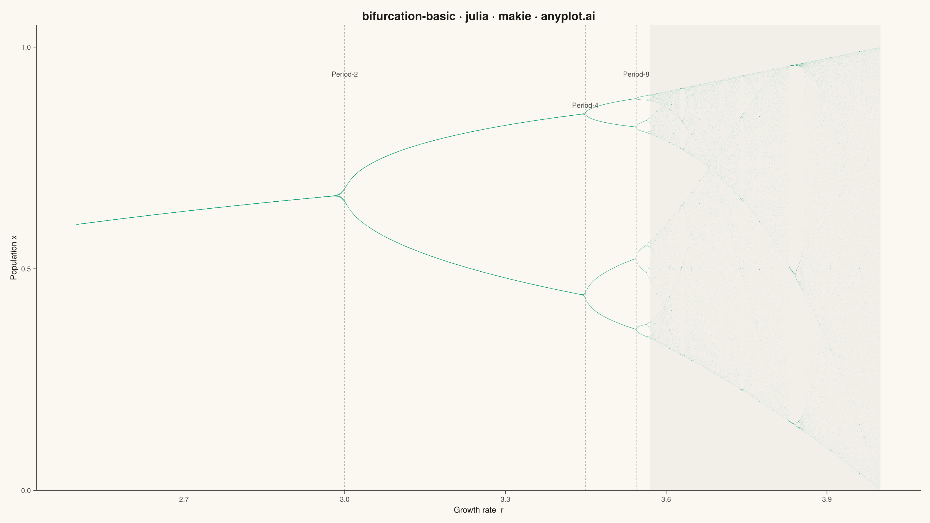
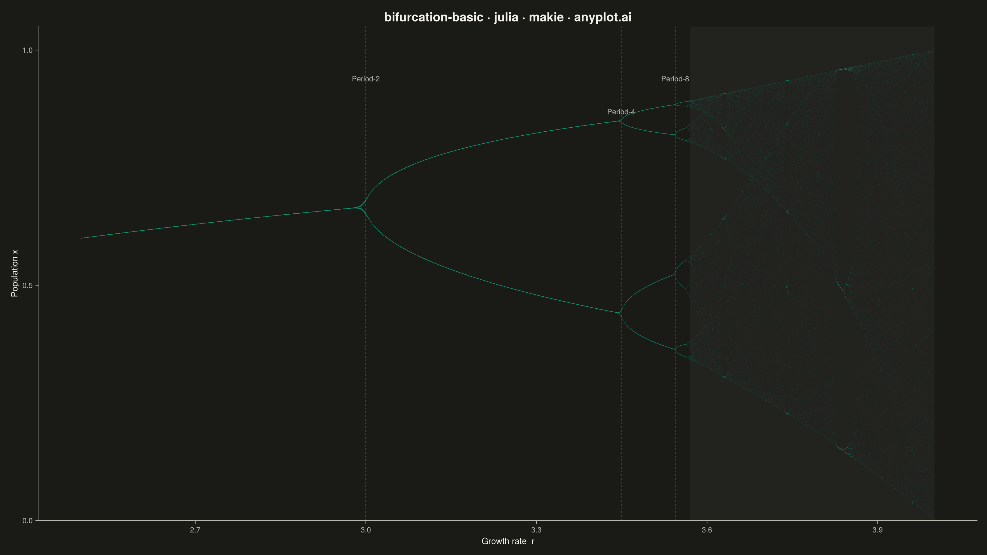
A bifurcation diagram shows how the steady-state behavior of a dynamical system changes as a control parameter varies. By plotting the long-term values of a state variable against a continuously varied parameter, it reveals transitions from stable fixed points through period-doubling cascades to chaotic regimes. The classic example is the logistic map, where the route to chaos is clearly visible as the growth rate parameter increases.
# anyplot.ai
# bifurcation-basic: Bifurcation Diagram for Dynamical Systems
# Library: makie 0.22.10 | Julia 1.11.9
# Quality: 91/100 | Created: 2026-06-17

using CairoMakie
using Colors
using Random

Random.seed!(42)

# Theme tokens
const THEME    = get(ENV, "ANYPLOT_THEME", "light")
const PAGE_BG  = THEME == "light" ? colorant"#FAF8F1" : colorant"#1A1A17"
const INK      = THEME == "light" ? colorant"#1A1A17" : colorant"#F0EFE8"
const INK_SOFT = THEME == "light" ? colorant"#4A4A44" : colorant"#B8B7B0"

const IMPRINT_PALETTE = [
    colorant"#009E73",
    colorant"#C475FD",
    colorant"#4467A3",
    colorant"#BD8233",
    colorant"#AE3030",
    colorant"#2ABCCD",
    colorant"#954477",
    colorant"#99B314",
]

# Data — logistic map: x(n+1) = r * x(n) * (1 - x(n))
n_r    = 2000
n_warm = 200
n_keep = 100

r_values = LinRange(2.5, 4.0, n_r)
r_pts    = Float64[]
x_pts    = Float64[]
sizehint!(r_pts, n_r * n_keep)
sizehint!(x_pts, n_r * n_keep)

for r in r_values
    x = 0.5
    for _ in 1:n_warm
        x = r * x * (1.0 - x)
    end
    for _ in 1:n_keep
        x = r * x * (1.0 - x)
        push!(r_pts, r)
        push!(x_pts, x)
    end
end

# Custom Makie theme — anyplot chrome tokens applied via with_theme
anyplot_theme = Theme(
    fontsize = 14,
    Axis = (
        backgroundcolor   = PAGE_BG,
        titlecolor        = INK,
        titlesize         = 20,
        xlabelcolor       = INK,
        ylabelcolor       = INK,
        xlabelsize        = 14,
        ylabelsize        = 14,
        xticklabelcolor   = INK_SOFT,
        yticklabelcolor   = INK_SOFT,
        xticklabelsize    = 12,
        yticklabelsize    = 12,
        xtickcolor        = INK_SOFT,
        ytickcolor        = INK_SOFT,
        leftspinecolor    = INK_SOFT,
        bottomspinecolor  = INK_SOFT,
        topspinevisible   = false,
        rightspinevisible = false,
        xgridvisible      = false,
        ygridvisible      = false,
    ),
)

with_theme(anyplot_theme) do
    fig = Figure(
        size            = (1600, 900),
        backgroundcolor = PAGE_BG,
    )

    ax = Axis(
        fig[1, 1];
        title  = "bifurcation-basic · julia · makie · anyplot.ai",
        xlabel = "Growth rate  r",
        ylabel = "Population x",
    )

    # Subtle shading for the chaotic regime (Feigenbaum onset r ≈ 3.57)
    chaotic_poly = Point2f[(3.57, 0.0), (4.0, 0.0), (4.0, 1.05), (3.57, 1.05)]
    poly!(ax, chaotic_poly; color = (INK, 0.04), strokewidth = 0)

    # Density scatter — slightly higher alpha for dark theme to preserve contrast
    pt_alpha = THEME == "dark" ? 0.13 : 0.10
    scatter!(ax, r_pts, x_pts;
        color       = (IMPRINT_PALETTE[1], pt_alpha),
        markersize  = 1.0,
        strokewidth = 0,
    )

    ylims!(ax, 0.0, 1.05)

    # Bifurcation point labels — period-doubling cascade
    bif_r      = [3.0,        3.449,      3.544]
    bif_labels = ["Period-2", "Period-4", "Period-8"]
    bif_y      = [0.93,       0.86,       0.93]

    for (r_val, label, y_pos) in zip(bif_r, bif_labels, bif_y)
        vlines!(ax, [r_val];
            color     = (INK_SOFT, 0.5),
            linewidth = 1.0,
            linestyle = :dash,
        )
        text!(ax, label;
            position = (r_val, y_pos),
            align    = (:center, :bottom),
            fontsize = 12,
            color    = INK_SOFT,
        )
    end

    save("plot-$(THEME).png", fig; px_per_unit = 2)
end
Runnable source as JSON, for any HTTP client: https://api.anyplot.ai/specs/bifurcation-basic/makie/code. Any spec id and library id listed in llms-full.txt fit the same URL shape; every URL below is complete and callable.
{
  "spec_id": "bifurcation-basic",
  "language": "julia",
  "library": "makie",
  "page": "https://anyplot.ai/bifurcation-basic/julia/makie",
  "hub": "https://anyplot.ai/bifurcation-basic",
  "code_json": "https://api.anyplot.ai/specs/bifurcation-basic/makie/code",
  "spec_json": "https://api.anyplot.ai/specs/bifurcation-basic",
  "render_light_png": "https://storage.googleapis.com/anyplot-images/plots/bifurcation-basic/julia/makie/plot-light.png",
  "render_dark_png": "https://storage.googleapis.com/anyplot-images/plots/bifurcation-basic/julia/makie/plot-dark.png",
  "quality_score": 91.0,
  "license": "MIT",
  "guide": "https://anyplot.ai/llms.txt"
}
Part of Bifurcation Diagram for Dynamical Systems on anyplot.ai.