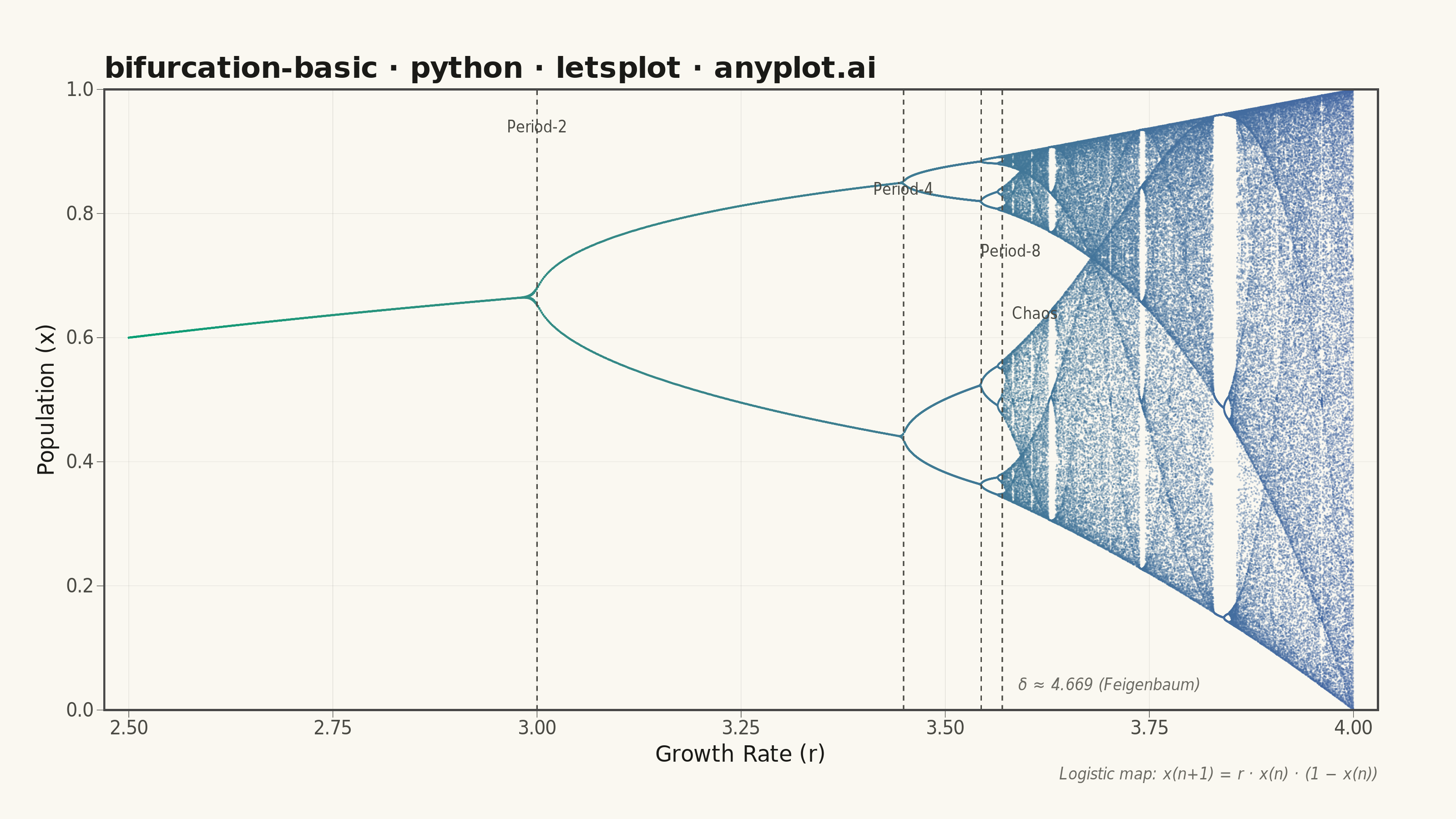
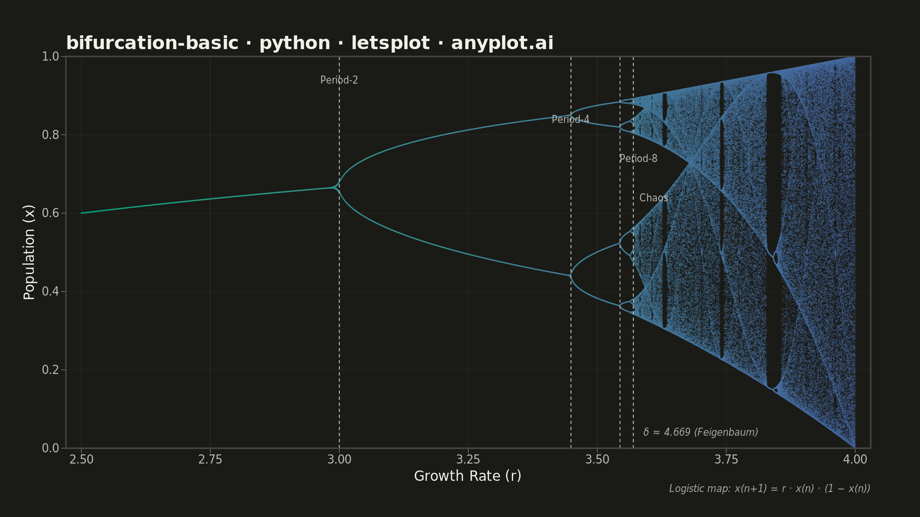
A bifurcation diagram shows how the steady-state behavior of a dynamical system changes as a control parameter varies. By plotting the long-term values of a state variable against a continuously varied parameter, it reveals transitions from stable fixed points through period-doubling cascades to chaotic regimes. The classic example is the logistic map, where the route to chaos is clearly visible as the growth rate parameter increases.
""" anyplot.ai
bifurcation-basic: Bifurcation Diagram for Dynamical Systems
Library: letsplot 4.10.1 | Python 3.13.14
Quality: 92/100 | Updated: 2026-06-17
"""

import os

import numpy as np
import pandas as pd
from lets_plot import (
    LetsPlot,
    aes,
    coord_cartesian,
    element_blank,
    element_line,
    element_rect,
    element_text,
    geom_point,
    geom_segment,
    geom_text,
    ggplot,
    ggsave,
    ggsize,
    guides,
    labs,
    sampling_pick,
    scale_color_gradient,
    scale_x_continuous,
    scale_y_continuous,
    theme,
    theme_minimal,
)


LetsPlot.setup_html()

THEME = os.getenv("ANYPLOT_THEME", "light")

# Theme-adaptive chrome tokens
PAGE_BG = "#FAF8F1" if THEME == "light" else "#1A1A17"
ELEVATED_BG = "#FFFDF6" if THEME == "light" else "#242420"
INK = "#1A1A17" if THEME == "light" else "#F0EFE8"
INK_SOFT = "#4A4A44" if THEME == "light" else "#B8B7B0"
INK_MUTED = "#6B6A63" if THEME == "light" else "#A8A79F"
GRID_COLOR = "rgba(26, 26, 23, 0.15)" if THEME == "light" else "rgba(240, 239, 232, 0.15)"

# Imprint sequential colormap: brand green → blue (single-polarity continuous)
IMPRINT_SEQ_LOW = "#009E73"
IMPRINT_SEQ_HIGH = "#4467A3"

# Data — Logistic map: x(n+1) = r * x(n) * (1 - x(n))
# Denser sampling in the chaotic regime for richer visualization
r_stable = np.linspace(2.5, 3.45, 600)
r_chaotic = np.linspace(3.45, 4.0, 1600)
r_values = np.concatenate([r_stable, r_chaotic])
transient = 250
iterations = 100

r_all = []
x_all = []

for r in r_values:
    x = 0.5
    for _ in range(transient):
        x = r * x * (1.0 - x)
    for _ in range(iterations):
        x = r * x * (1.0 - x)
        r_all.append(r)
        x_all.append(x)

df = pd.DataFrame({"r": np.array(r_all), "x": np.array(x_all)})

# Key bifurcation points with dashed guide lines
bif_r = [3.0, 3.449, 3.544, 3.5699]
segments_df = pd.DataFrame({"r": bif_r, "ymin": [0.0] * 4, "ymax": [1.0] * 4})

# Stagger labels at different y positions to avoid overlap
labels_df = pd.DataFrame(
    {
        "r": [3.0, 3.449, 3.58, 3.61],
        "x": [0.93, 0.83, 0.73, 0.63],
        "label": ["Period-2", "Period-4", "Period-8", "Chaos"],
    }
)

# Feigenbaum constant annotation near onset of chaos
feigen_df = pd.DataFrame({"r": [3.5699], "x": [0.05], "label": ["δ ≈ 4.669 (Feigenbaum)"]})

plot = (
    ggplot(df, aes(x="r", y="x", color="r"))
    + geom_point(size=0.4, alpha=0.35, tooltips="none", show_legend=False, sampling=sampling_pick(n=220000))
    # Imprint sequential colormap for the continuous r parameter
    + scale_color_gradient(low=IMPRINT_SEQ_LOW, high=IMPRINT_SEQ_HIGH, guide="none")
    + geom_segment(
        aes(x="r", y="ymin", xend="r", yend="ymax"),
        data=segments_df,
        color=INK_SOFT,
        size=0.3,
        linetype="dashed",
        inherit_aes=False,
        tooltips="none",
    )
    + geom_text(
        aes(x="r", y="x", label="label"), data=labels_df, size=4, color=INK_SOFT, hjust=0.5, vjust=0, inherit_aes=False
    )
    + geom_text(
        aes(x="r", y="x", label="label"),
        data=feigen_df,
        size=4.5,
        color=INK_MUTED,
        hjust=0,
        vjust=1,
        fontface="italic",
        nudge_x=0.02,
        inherit_aes=False,
    )
    + guides(color="none")
    + labs(
        x="Growth Rate (r)",
        y="Population (x)",
        title="bifurcation-basic · python · letsplot · anyplot.ai",
        caption="Logistic map: x(n+1) = r · x(n) · (1 − x(n))",
    )
    + scale_x_continuous(breaks=[2.5, 2.75, 3.0, 3.25, 3.5, 3.75, 4.0], expand=[0.02, 0], format=".2f")
    + scale_y_continuous(breaks=[0.0, 0.2, 0.4, 0.6, 0.8, 1.0], expand=[0.02, 0], format=".1f")
    + coord_cartesian(ylim=[0, 1])
    # Canvas: ggsize(800, 450) × scale=4 → 3200×1800 px (landscape)
    + ggsize(800, 450)
    + theme_minimal()
    + theme(
        axis_text=element_text(size=10, color=INK_SOFT),
        axis_title=element_text(size=12, color=INK),
        plot_title=element_text(size=16, color=INK, face="bold"),
        plot_caption=element_text(size=9, color=INK_MUTED, face="italic"),
        panel_grid_major_x=element_line(color=GRID_COLOR, size=0.2),
        panel_grid_major_y=element_line(color=GRID_COLOR, size=0.15),
        panel_grid_minor=element_blank(),
        plot_background=element_rect(fill=PAGE_BG, color=PAGE_BG),
        panel_background=element_rect(fill=PAGE_BG),
        axis_ticks=element_line(color=INK_SOFT, size=0.3),
        axis_line=element_line(color=INK_SOFT, size=0.4),
        plot_margin=[30, 40, 20, 20],
    )
)

# Save PNG (scale=4 → 3200×1800 px) and interactive HTML
ggsave(plot, f"plot-{THEME}.png", path=".", scale=4)
ggsave(plot, f"plot-{THEME}.html", path=".")
Runnable source as JSON, for any HTTP client: https://api.anyplot.ai/specs/bifurcation-basic/letsplot/code. Any spec id and library id listed in llms-full.txt fit the same URL shape; every URL below is complete and callable.
{
  "spec_id": "bifurcation-basic",
  "language": "python",
  "library": "letsplot",
  "page": "https://anyplot.ai/bifurcation-basic/python/letsplot",
  "hub": "https://anyplot.ai/bifurcation-basic",
  "code_json": "https://api.anyplot.ai/specs/bifurcation-basic/letsplot/code",
  "spec_json": "https://api.anyplot.ai/specs/bifurcation-basic",
  "render_light_png": "https://storage.googleapis.com/anyplot-images/plots/bifurcation-basic/python/letsplot/plot-light.png",
  "render_dark_png": "https://storage.googleapis.com/anyplot-images/plots/bifurcation-basic/python/letsplot/plot-dark.png",
  "interactive_light_html": "https://storage.googleapis.com/anyplot-images/plots/bifurcation-basic/python/letsplot/plot-light.html",
  "interactive_dark_html": "https://storage.googleapis.com/anyplot-images/plots/bifurcation-basic/python/letsplot/plot-dark.html",
  "quality_score": 92.0,
  "license": "MIT",
  "guide": "https://anyplot.ai/llms.txt"
}
Part of Bifurcation Diagram for Dynamical Systems on anyplot.ai.