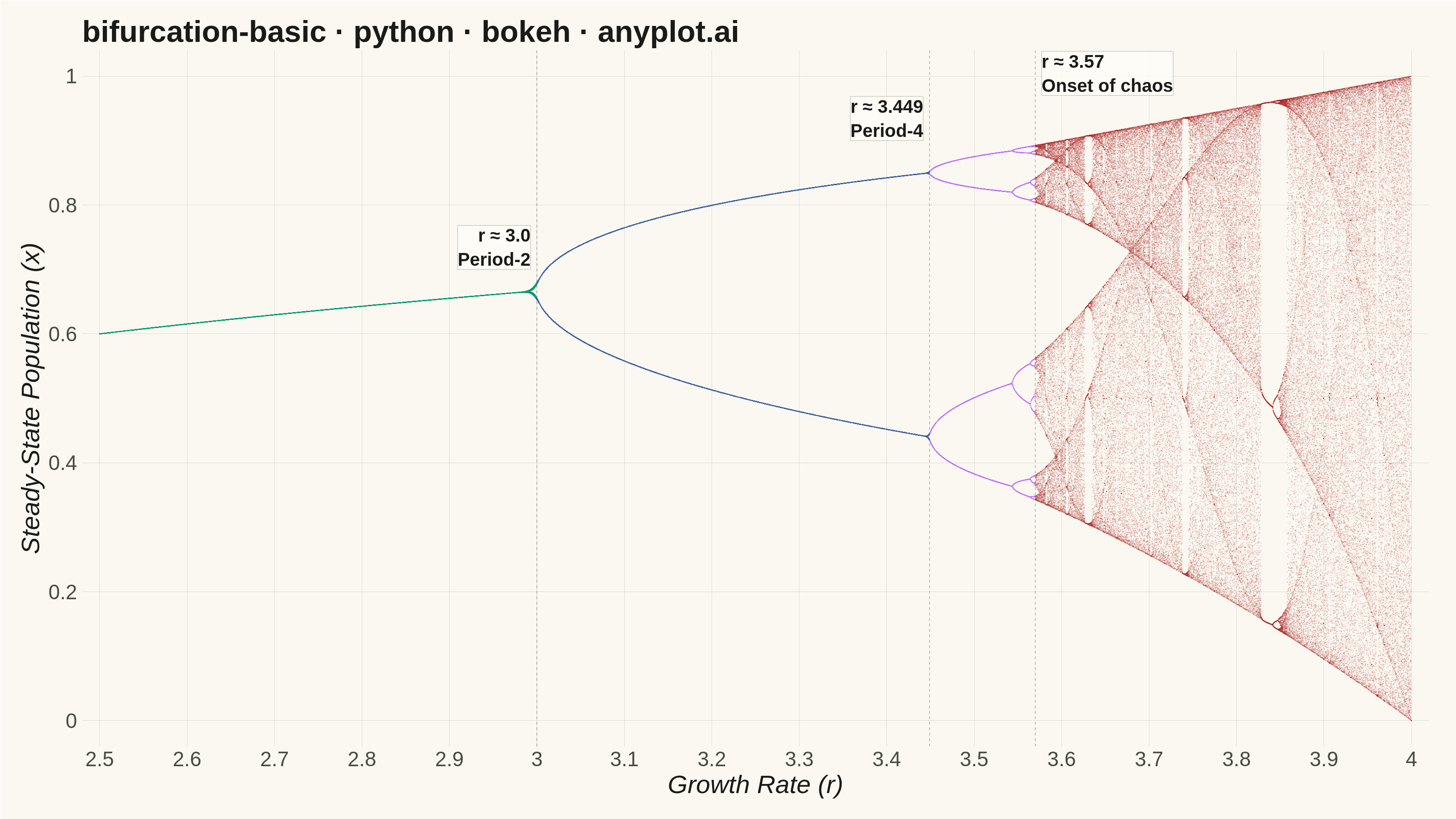
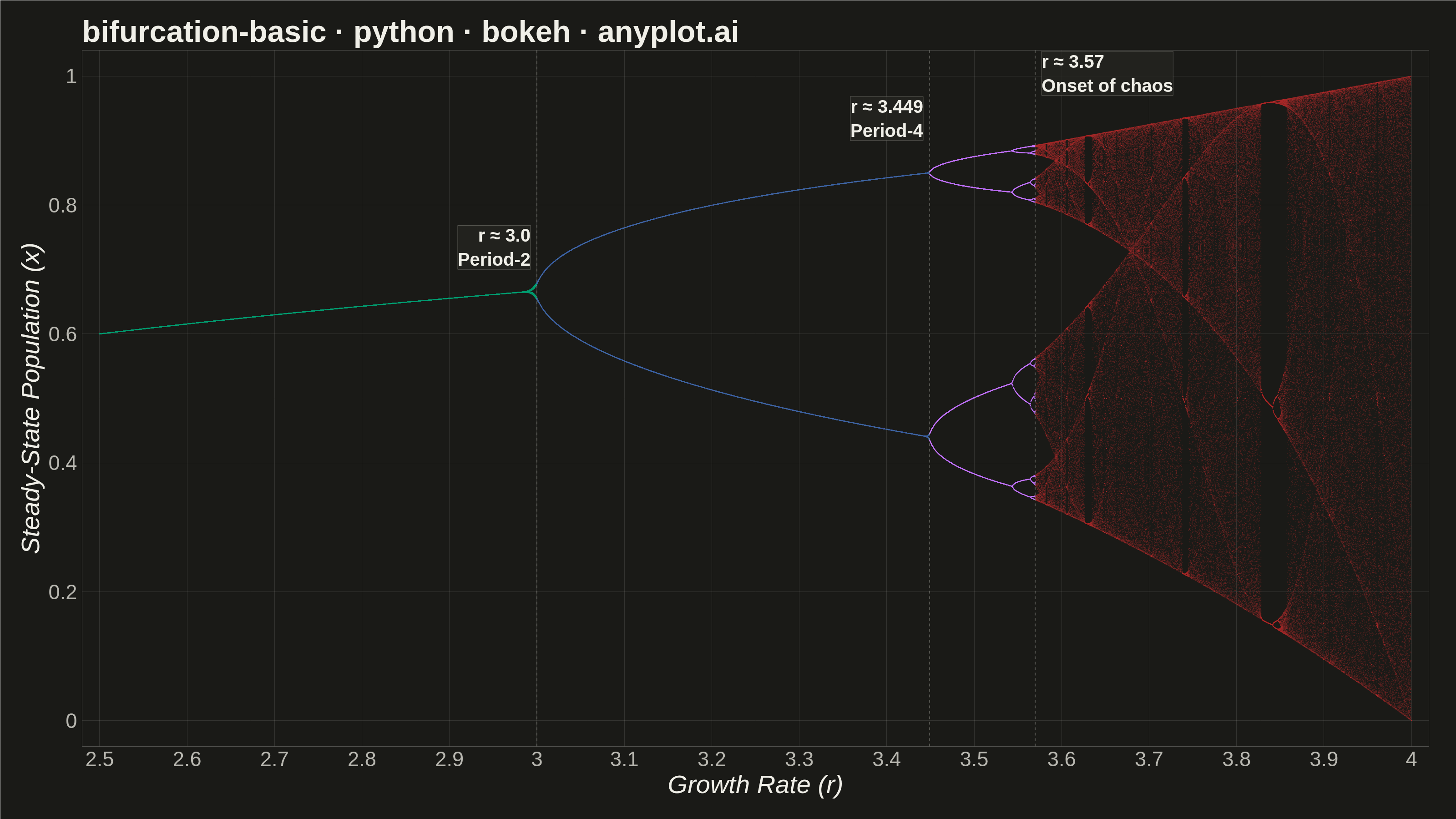
A bifurcation diagram shows how the steady-state behavior of a dynamical system changes as a control parameter varies. By plotting the long-term values of a state variable against a continuously varied parameter, it reveals transitions from stable fixed points through period-doubling cascades to chaotic regimes. The classic example is the logistic map, where the route to chaos is clearly visible as the growth rate parameter increases.
""" anyplot.ai
bifurcation-basic: Bifurcation Diagram for Dynamical Systems
Library: bokeh 3.9.1 | Python 3.13.13
Quality: 93/100 | Updated: 2026-06-17
"""

import os
import time
from pathlib import Path

import numpy as np
from bokeh.io import output_file, save
from bokeh.models import HoverTool, Label, Range1d, Span
from bokeh.plotting import ColumnDataSource, figure
from selenium import webdriver
from selenium.webdriver.chrome.options import Options


# Theme-adaptive chrome
THEME = os.getenv("ANYPLOT_THEME", "light")
PAGE_BG = "#FAF8F1" if THEME == "light" else "#1A1A17"
ELEVATED_BG = "#FFFDF6" if THEME == "light" else "#242420"
INK = "#1A1A17" if THEME == "light" else "#F0EFE8"
INK_SOFT = "#4A4A44" if THEME == "light" else "#B8B7B0"

# Imprint palette — regime encoding tells the route-to-chaos story.
# Semantic ordering: stable=brand green, intermediate periods cool blue/lavender,
# chaos=matte-red (Imprint semantic anchor for instability). First series #009E73.
IMPRINT_STABLE = "#009E73"  # position 1 — stable fixed point (good/safe → green)
IMPRINT_PERIOD2 = "#4467A3"  # position 3 — period-2 band
IMPRINT_PERIOD4 = "#C475FD"  # position 2 — period-4 / higher period
IMPRINT_CHAOS = "#AE3030"  # position 5 — chaotic regime (instability → red anchor)

# Data — logistic map: x(n+1) = r * x(n) * (1 - x(n))
r_min, r_max = 2.5, 4.0
n_r = 3000
n_transient = 300
n_keep = 150

r_values = np.linspace(r_min, r_max, n_r)
all_r = np.repeat(r_values, n_keep)
all_x = np.empty_like(all_r)

idx = 0
for r in r_values:
    x = 0.5
    for _ in range(n_transient):
        x = r * x * (1.0 - x)
    for _ in range(n_keep):
        x = r * x * (1.0 - x)
        all_x[idx] = x
        idx += 1

# Vectorized regime-based color + density-aware alpha (np.select, no Python loop).
# Chaos alpha lifted from the old 0.15 to 0.30 so the dense red fractal holds
# contrast on both the cream and near-black surfaces.
r_cuts = [all_r < 3.0, all_r < 3.449, all_r < 3.5699]
colors = np.select(r_cuts, [IMPRINT_STABLE, IMPRINT_PERIOD2, IMPRINT_PERIOD4], default=IMPRINT_CHAOS)
alphas = np.select(r_cuts, [0.65, 0.50, 0.40], default=0.30)

source = ColumnDataSource(data={"r": all_r, "x": all_x, "color": colors, "alpha": alphas})

# Plot — canonical 3200×1800 landscape canvas
title = "bifurcation-basic · python · bokeh · anyplot.ai"
p = figure(
    width=3200,
    height=1800,
    title=title,
    x_axis_label="Growth Rate (r)",
    y_axis_label="Steady-State Population (x)",
    x_range=Range1d(r_min - 0.02, r_max + 0.02),
    y_range=Range1d(-0.04, 1.04),
    toolbar_location=None,
    min_border_bottom=160,
    min_border_left=180,
    min_border_top=110,
    min_border_right=60,
    tools="pan,wheel_zoom,box_zoom,reset,save",
    active_scroll="wheel_zoom",
)

scatter = p.scatter(x="r", y="x", source=source, size=2, color="color", alpha="alpha", line_color=None)

# HoverTool — Bokeh-distinctive interactive feature (live in the HTML artifact)
hover = HoverTool(
    renderers=[scatter], tooltips=[("r", "@r{0.000}"), ("x", "@x{0.0000}")], point_policy="snap_to_data", mode="mouse"
)
p.add_tools(hover)

# Vertical guides at the key bifurcation points
bif_points = [3.0, 3.449, 3.5699]
for r_bif in bif_points:
    p.add_layout(
        Span(location=r_bif, dimension="height", line_color=INK_SOFT, line_width=2, line_alpha=0.35, line_dash="dashed")
    )

# Annotations — boxed so they read over the dense chaotic fan; the chaos label
# now sits high inside the structure it describes instead of floating at y≈0.05.
annotations = [
    (3.0, 0.70, "r ≈ 3.0\nPeriod-2", "right"),
    (3.449, 0.90, "r ≈ 3.449\nPeriod-4", "right"),
    (3.5699, 0.97, "r ≈ 3.57\nOnset of chaos", "left"),
]
for r_bif, y_pos, label_text, align in annotations:
    p.add_layout(
        Label(
            x=r_bif,
            y=y_pos,
            text=label_text,
            text_font_size="30pt",
            text_font_style="bold",
            text_color=INK,
            text_align=align,
            x_offset=14 if align == "left" else -14,
            background_fill_color=ELEVATED_BG,
            background_fill_alpha=0.82,
            border_line_color=INK_SOFT,
            border_line_alpha=0.4,
        )
    )

# Style — typography
p.title.text_font_size = "50pt"
p.title.text_color = INK
p.xaxis.axis_label_text_font_size = "42pt"
p.yaxis.axis_label_text_font_size = "42pt"
p.xaxis.major_label_text_font_size = "34pt"
p.yaxis.major_label_text_font_size = "34pt"
p.xaxis.axis_label_text_color = INK
p.yaxis.axis_label_text_color = INK
p.xaxis.major_label_text_color = INK_SOFT
p.yaxis.major_label_text_color = INK_SOFT

# Chrome — clean L-frame, ticks/axis lines removed for a minimal scatter
p.xaxis.axis_line_color = None
p.yaxis.axis_line_color = None
p.xaxis.major_tick_line_color = None
p.yaxis.major_tick_line_color = None
p.xaxis.minor_tick_line_color = None
p.yaxis.minor_tick_line_color = None

p.xgrid.grid_line_color = INK
p.ygrid.grid_line_color = INK
p.xgrid.grid_line_alpha = 0.12
p.ygrid.grid_line_alpha = 0.12

p.background_fill_color = PAGE_BG
p.border_fill_color = PAGE_BG
p.outline_line_color = None

p.xaxis.ticker.desired_num_ticks = 12
p.yaxis.ticker.desired_num_ticks = 8

# Save — interactive HTML artifact + headless-Chrome screenshot at the exact canvas size
output_file(f"plot-{THEME}.html", title="Bifurcation Diagram")
save(p)

W, H = 3200, 1800
opts = Options()
for arg in (
    "--headless=new",
    "--no-sandbox",
    "--disable-dev-shm-usage",
    "--disable-gpu",
    f"--window-size={W},{H}",
    "--hide-scrollbars",
):
    opts.add_argument(arg)
driver = webdriver.Chrome(options=opts)
driver.set_window_size(W, H)
driver.get(f"file://{Path(f'plot-{THEME}.html').resolve()}")
time.sleep(3)  # let bokeh's JS render the canvas

# Headless Chrome reserves a strip of window chrome, so the inner viewport (what
# save_screenshot captures) lands ~140px short of the requested window height.
# Measure the delta and resize so the viewport is EXACTLY 3200×1800.
inner_w, inner_h = driver.execute_script("return [window.innerWidth, window.innerHeight];")
driver.set_window_size(W + (W - inner_w), H + (H - inner_h))
time.sleep(1)

driver.save_screenshot(f"plot-{THEME}.png")
driver.quit()
Runnable source as JSON, for any HTTP client: https://api.anyplot.ai/specs/bifurcation-basic/bokeh/code. Any spec id and library id listed in llms-full.txt fit the same URL shape; every URL below is complete and callable.
{
  "spec_id": "bifurcation-basic",
  "language": "python",
  "library": "bokeh",
  "page": "https://anyplot.ai/bifurcation-basic/python/bokeh",
  "hub": "https://anyplot.ai/bifurcation-basic",
  "code_json": "https://api.anyplot.ai/specs/bifurcation-basic/bokeh/code",
  "spec_json": "https://api.anyplot.ai/specs/bifurcation-basic",
  "render_light_png": "https://storage.googleapis.com/anyplot-images/plots/bifurcation-basic/python/bokeh/plot-light.png",
  "render_dark_png": "https://storage.googleapis.com/anyplot-images/plots/bifurcation-basic/python/bokeh/plot-dark.png",
  "interactive_light_html": "https://storage.googleapis.com/anyplot-images/plots/bifurcation-basic/python/bokeh/plot-light.html",
  "interactive_dark_html": "https://storage.googleapis.com/anyplot-images/plots/bifurcation-basic/python/bokeh/plot-dark.html",
  "quality_score": 93.0,
  "license": "MIT",
  "guide": "https://anyplot.ai/llms.txt"
}
Part of Bifurcation Diagram for Dynamical Systems on anyplot.ai.