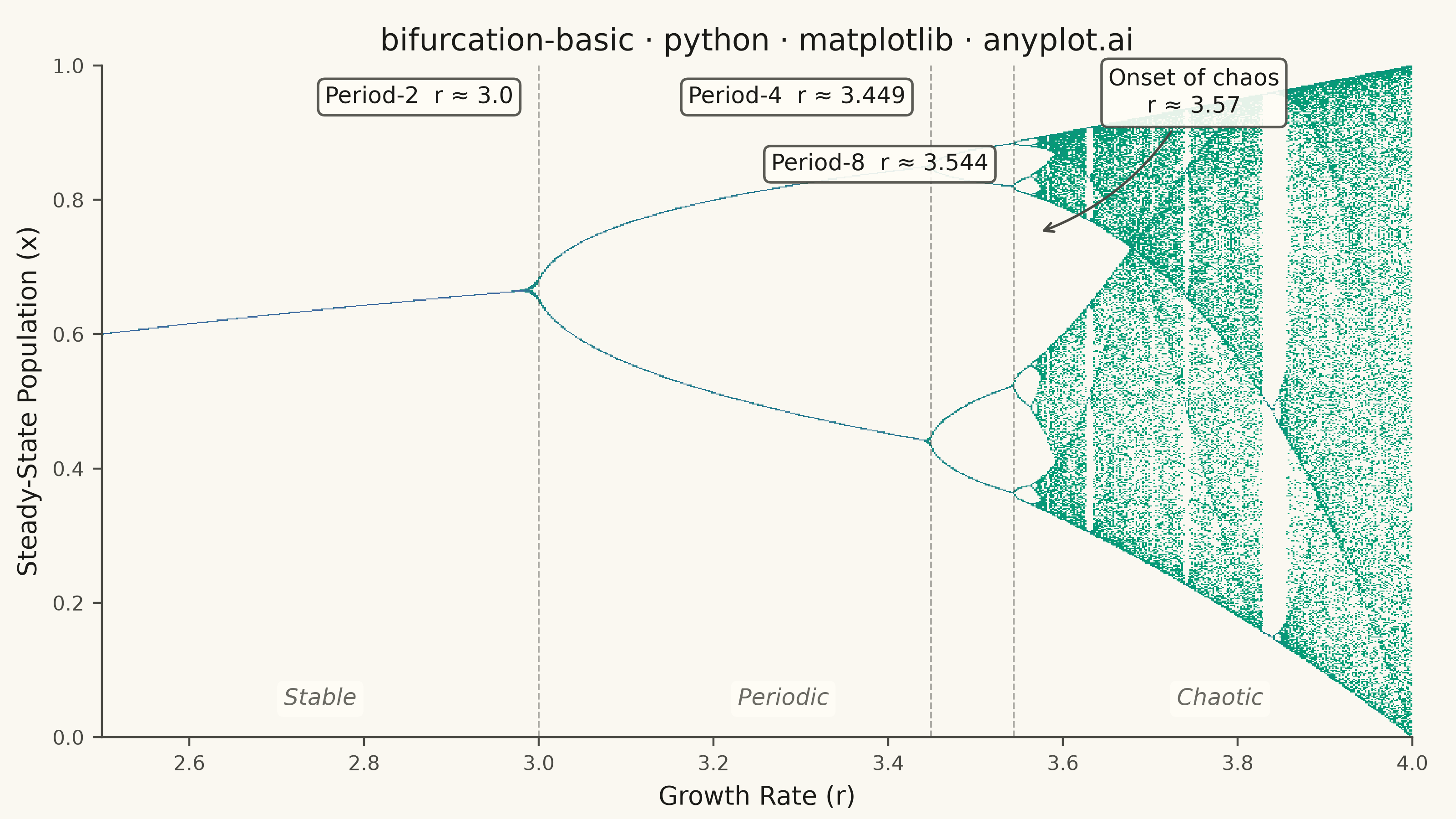
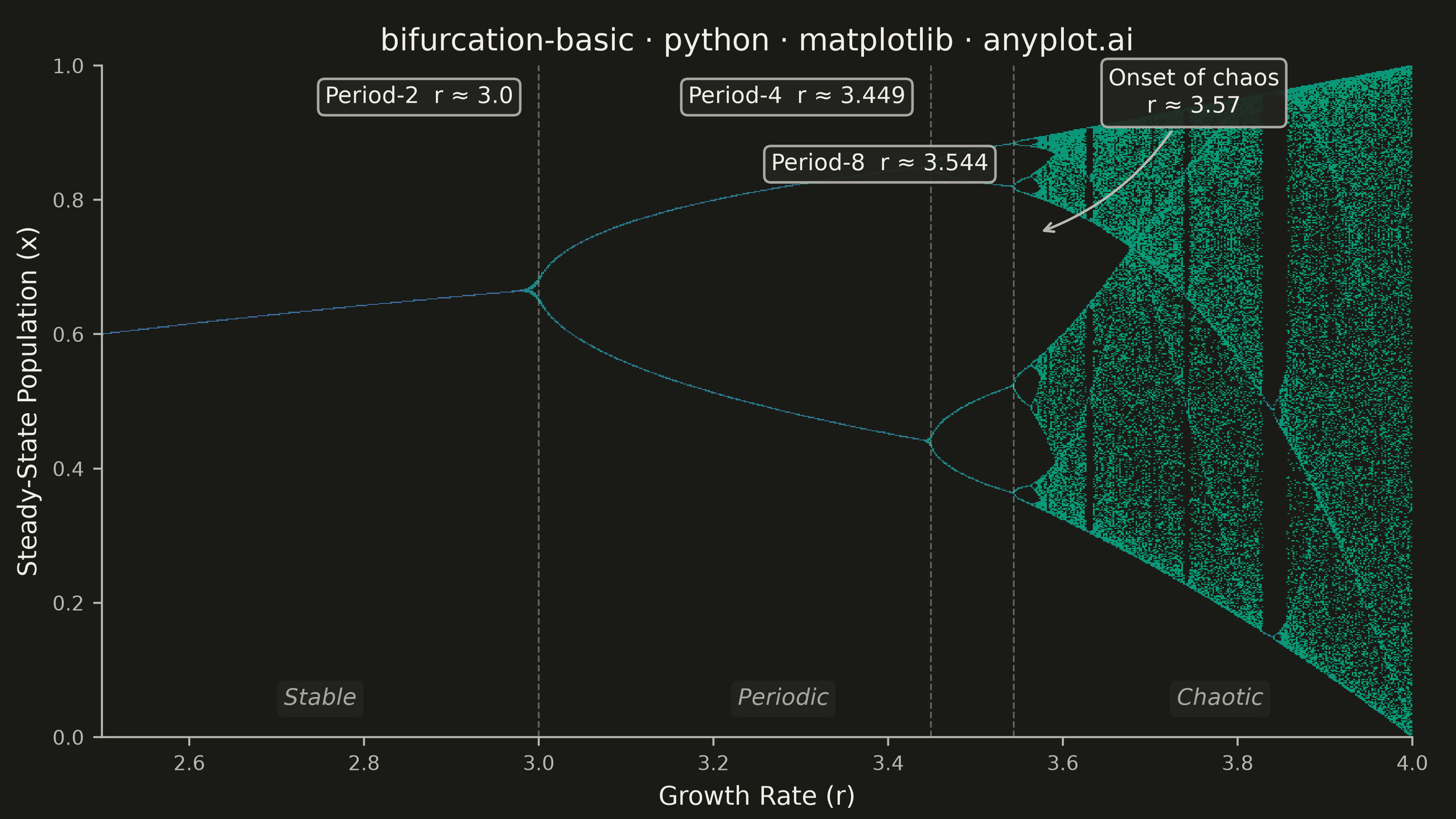
A bifurcation diagram shows how the steady-state behavior of a dynamical system changes as a control parameter varies. By plotting the long-term values of a state variable against a continuously varied parameter, it reveals transitions from stable fixed points through period-doubling cascades to chaotic regimes. The classic example is the logistic map, where the route to chaos is clearly visible as the growth rate parameter increases.
""" anyplot.ai
bifurcation-basic: Bifurcation Diagram for Dynamical Systems
Library: matplotlib 3.11.0 | Python 3.13.13
Quality: 92/100 | Updated: 2026-06-17
"""

import os

import matplotlib.pyplot as plt
import numpy as np
from matplotlib.colors import LinearSegmentedColormap, PowerNorm


# Theme-adaptive chrome
THEME = os.getenv("ANYPLOT_THEME", "light")
PAGE_BG = "#FAF8F1" if THEME == "light" else "#1A1A17"
ELEVATED_BG = "#FFFDF6" if THEME == "light" else "#242420"
INK = "#1A1A17" if THEME == "light" else "#F0EFE8"
INK_SOFT = "#4A4A44" if THEME == "light" else "#B8B7B0"
INK_MUTED = "#6B6A63" if THEME == "light" else "#A8A79F"

# Continuous density → Imprint sequential cmap (brand green → blue).
# Empty bins render as the page background so the diagram floats on the surface.
imprint_seq = LinearSegmentedColormap.from_list("imprint_seq", ["#009E73", "#4467A3"])
imprint_seq.set_bad(PAGE_BG)

# Data — logistic map x(n+1) = r * x(n) * (1 - x(n))
r_min, r_max = 2.5, 4.0
num_r = 2000
transient = 200
iterations = 100

r_values = np.linspace(r_min, r_max, num_r)
r_plot = np.empty(num_r * iterations)
x_plot = np.empty(num_r * iterations)

for i, r in enumerate(r_values):
    x = 0.5
    for _ in range(transient):
        x = r * x * (1 - x)
    for j in range(iterations):
        x = r * x * (1 - x)
        r_plot[i * iterations + j] = r
        x_plot[i * iterations + j] = x

# 2D histogram for density-based rendering of the attractor structure.
# Reveals periodic windows within chaos far better than a raw scatter.
r_bins = 800
x_bins = 600
hist, r_edges, x_edges = np.histogram2d(r_plot, x_plot, bins=[r_bins, x_bins], range=[[r_min, r_max], [0, 1]])
hist = np.ma.masked_where(hist == 0, hist)

# Plot
fig, ax = plt.subplots(figsize=(8, 4.5), dpi=400, facecolor=PAGE_BG)
ax.set_facecolor(PAGE_BG)

# Density heatmap; PowerNorm lifts low-density branches into visibility.
ax.pcolormesh(
    r_edges,
    x_edges,
    hist.T,
    cmap=imprint_seq,
    norm=PowerNorm(gamma=0.40, vmin=1, vmax=hist.max()),
    rasterized=True,
    zorder=1,
)

# Regime labels at the bottom carry the stability → chaos narrative.
label_bbox = {"boxstyle": "round,pad=0.3", "facecolor": ELEVATED_BG, "edgecolor": "none", "alpha": 0.85}
for rx, label in [(2.75, "Stable"), (3.28, "Periodic"), (3.78, "Chaotic")]:
    ax.text(
        rx,
        0.04,
        label,
        transform=ax.get_xaxis_transform(),
        fontsize=9,
        color=INK_MUTED,
        ha="center",
        va="bottom",
        fontstyle="italic",
        bbox=label_bbox,
        zorder=3,
    )

# Key period-doubling bifurcations — dashed markers with spaced callouts.
ann_bbox = {"boxstyle": "round,pad=0.3", "facecolor": ELEVATED_BG, "edgecolor": INK_SOFT, "alpha": 0.9}
bifurcation_points = [(3.0, "Period-2", -10, 0.97), (3.449, "Period-4", -10, 0.97), (3.544, "Period-8", -10, 0.87)]
for r_bif, label, x_offset, y_frac in bifurcation_points:
    ax.axvline(r_bif, color=INK_SOFT, linewidth=0.7, linestyle="--", alpha=0.45, zorder=2)
    ax.annotate(
        f"{label}  r ≈ {r_bif}",
        xy=(r_bif, y_frac),
        xycoords=("data", "axes fraction"),
        xytext=(x_offset, 0),
        textcoords="offset points",
        fontsize=9,
        color=INK,
        ha="right",
        va="top",
        bbox=ann_bbox,
        zorder=4,
    )

# Onset of chaos
ax.annotate(
    "Onset of chaos\nr ≈ 3.57",
    xy=(3.57, 0.75),
    xytext=(3.75, 0.93),
    fontsize=9,
    color=INK,
    ha="center",
    bbox=ann_bbox,
    arrowprops={"arrowstyle": "->", "color": INK_SOFT, "connectionstyle": "arc3,rad=-0.2"},
    zorder=4,
)

# Style
ax.set_xlabel("Growth Rate (r)", fontsize=10, color=INK)
ax.set_ylabel("Steady-State Population (x)", fontsize=10, color=INK)
title = "bifurcation-basic · python · matplotlib · anyplot.ai"
ax.set_title(title, fontsize=12, fontweight="medium", color=INK)
ax.tick_params(axis="both", labelsize=8, colors=INK_SOFT, labelcolor=INK_SOFT)
ax.set_xlim(r_min, r_max)
ax.set_ylim(0, 1)
for s in ("left", "bottom"):
    ax.spines[s].set_color(INK_SOFT)
ax.spines["top"].set_visible(False)
ax.spines["right"].set_visible(False)

fig.subplots_adjust(left=0.07, right=0.97, top=0.92, bottom=0.10)
plt.savefig(f"plot-{THEME}.png", dpi=400, facecolor=PAGE_BG)
Runnable source as JSON, for any HTTP client: https://api.anyplot.ai/specs/bifurcation-basic/matplotlib/code. Any spec id and library id listed in llms-full.txt fit the same URL shape; every URL below is complete and callable.
{
  "spec_id": "bifurcation-basic",
  "language": "python",
  "library": "matplotlib",
  "page": "https://anyplot.ai/bifurcation-basic/python/matplotlib",
  "hub": "https://anyplot.ai/bifurcation-basic",
  "code_json": "https://api.anyplot.ai/specs/bifurcation-basic/matplotlib/code",
  "spec_json": "https://api.anyplot.ai/specs/bifurcation-basic",
  "render_light_png": "https://storage.googleapis.com/anyplot-images/plots/bifurcation-basic/python/matplotlib/plot-light.png",
  "render_dark_png": "https://storage.googleapis.com/anyplot-images/plots/bifurcation-basic/python/matplotlib/plot-dark.png",
  "quality_score": 92.0,
  "license": "MIT",
  "guide": "https://anyplot.ai/llms.txt"
}
Part of Bifurcation Diagram for Dynamical Systems on anyplot.ai.