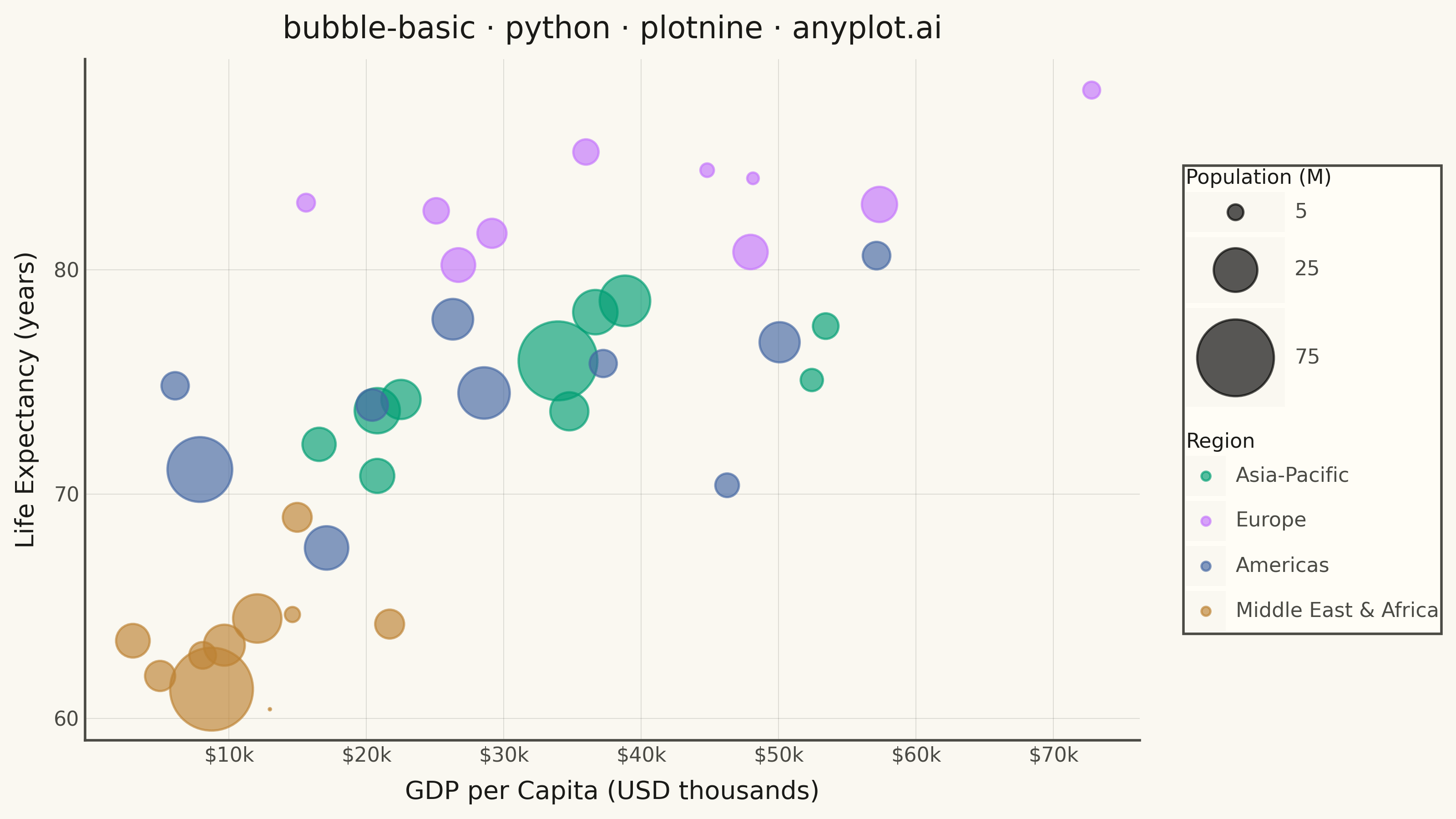
A bubble chart extending scatter plots by adding a third dimension through bubble size. Each point's position shows two variables (x, y) while the bubble size represents a third quantitative variable. This visualization is excellent for understanding relationships between three numerical variables simultaneously, revealing patterns that would be hidden in traditional 2D scatter plots.
""" anyplot.ai
bubble-basic: Basic Bubble Chart
Library: plotnine 0.15.4 | Python 3.13.13
Quality: 86/100 | Updated: 2026-05-28
"""

import os

import numpy as np
import pandas as pd
from plotnine import (
    aes,
    element_blank,
    element_line,
    element_rect,
    element_text,
    geom_point,
    geom_smooth,
    ggplot,
    labs,
    scale_color_manual,
    scale_size_area,
    scale_x_continuous,
    scale_y_continuous,
    theme,
    theme_minimal,
)


# Theme tokens
THEME = os.getenv("ANYPLOT_THEME", "light")
PAGE_BG = "#FAF8F1" if THEME == "light" else "#1A1A17"
ELEVATED_BG = "#FFFDF6" if THEME == "light" else "#242420"
INK = "#1A1A17" if THEME == "light" else "#F0EFE8"
INK_SOFT = "#4A4A44" if THEME == "light" else "#B8B7B0"
ANYPLOT_PALETTE = ["#009E73", "#C475FD", "#4467A3", "#BD8233", "#AE3030", "#2ABCCD", "#954477", "#99B314"]

# Data — countries across 4 regions: GDP per capita, life expectancy, population
np.random.seed(42)

regions = ["Asia-Pacific", "Europe", "Americas", "Middle East & Africa"]
region_params = {
    "Asia-Pacific": {"n": 10, "gdp_mean": 25, "gdp_std": 18, "le_base": 72, "pop_mean": 3.2},
    "Europe": {"n": 10, "gdp_mean": 45, "gdp_std": 15, "le_base": 78, "pop_mean": 2.0},
    "Americas": {"n": 10, "gdp_mean": 30, "gdp_std": 20, "le_base": 70, "pop_mean": 2.8},
    "Middle East & Africa": {"n": 10, "gdp_mean": 12, "gdp_std": 10, "le_base": 62, "pop_mean": 2.5},
}

rows = []
for region, p in region_params.items():
    gdp = np.abs(np.random.normal(p["gdp_mean"], p["gdp_std"], p["n"]))
    gdp = np.clip(gdp, 3, 85)
    le = p["le_base"] + 0.15 * gdp + np.random.normal(0, 2.5, p["n"])
    le = np.clip(le, 52, 88)
    pop = np.random.lognormal(mean=p["pop_mean"], sigma=0.8, size=p["n"])
    for i in range(p["n"]):
        rows.append({"gdp_per_capita": gdp[i], "life_expectancy": le[i], "population": pop[i], "region": region})

df = pd.DataFrame(rows)
df["region"] = pd.Categorical(df["region"], categories=regions, ordered=True)

# Plot
plot = (
    ggplot(df, aes(x="gdp_per_capita", y="life_expectancy", size="population", color="region"))
    + geom_smooth(
        aes(x="gdp_per_capita", y="life_expectancy"), method="lm", se=False, color=INK_SOFT, size=0.7, inherit_aes=False
    )
    + geom_point(alpha=0.65, stroke=0.4)
    + scale_size_area(max_size=18, breaks=[5, 25, 75], name="Population (M)")
    + scale_color_manual(values=ANYPLOT_PALETTE[:4], name="Region")
    + scale_x_continuous(labels=lambda lst: [f"${v:.0f}k" for v in lst], breaks=[10, 20, 30, 40, 50, 60, 70, 80])
    + scale_y_continuous(labels=lambda lst: [f"{v:.0f}" for v in lst])
    + labs(
        x="GDP per Capita (USD thousands)",
        y="Life Expectancy (years)",
        title="bubble-basic · python · plotnine · anyplot.ai",
    )
    + theme_minimal()
    + theme(
        figure_size=(8, 4.5),
        text=element_text(size=7, color=INK_SOFT),
        axis_title=element_text(size=10, color=INK),
        axis_text=element_text(size=8, color=INK_SOFT),
        plot_title=element_text(size=12, color=INK),
        legend_title=element_text(size=8, color=INK),
        legend_text=element_text(size=8, color=INK_SOFT),
        legend_key=element_rect(fill=PAGE_BG, color="none"),
        legend_background=element_rect(fill=ELEVATED_BG, color=INK_SOFT),
        panel_grid_major=element_line(color=INK, size=0.3, alpha=0.15),
        panel_grid_major_x=element_blank(),
        panel_grid_minor=element_blank(),
        plot_background=element_rect(fill=PAGE_BG, color=PAGE_BG),
        panel_background=element_rect(fill=PAGE_BG, color="none"),
        panel_border=element_blank(),
        axis_line=element_line(color=INK_SOFT),
    )
)

# Save
plot.save(f"plot-{THEME}.png", dpi=400, width=8, height=4.5, units="in", verbose=False)
Runnable source as JSON, for any HTTP client: https://api.anyplot.ai/specs/bubble-basic/plotnine/code. Any spec id and library id listed in llms-full.txt fit the same URL shape; every URL below is complete and callable.
{
  "spec_id": "bubble-basic",
  "language": "python",
  "library": "plotnine",
  "page": "https://anyplot.ai/bubble-basic/python/plotnine",
  "hub": "https://anyplot.ai/bubble-basic",
  "code_json": "https://api.anyplot.ai/specs/bubble-basic/plotnine/code",
  "spec_json": "https://api.anyplot.ai/specs/bubble-basic",
  "render_light_png": "https://storage.googleapis.com/anyplot-images/plots/bubble-basic/python/plotnine/plot-light.png",
  "render_dark_png": "https://storage.googleapis.com/anyplot-images/plots/bubble-basic/python/plotnine/plot-dark.png",
  "quality_score": 86.0,
  "license": "MIT",
  "guide": "https://anyplot.ai/llms.txt"
}
Part of Basic Bubble Chart on anyplot.ai.