The same plot in 14 other libraries — Python: Altair, Bokeh, lets-plot, Matplotlib, Plotly, plotnine, Pygal, Seaborn; Julia: Makie.jl; JavaScript: Chart.js, D3.js, Apache ECharts, Highcharts, MUI X Charts. Compare all 15 side by side: Basic Packed Bubble Chart in Python, R, Julia and JavaScript.
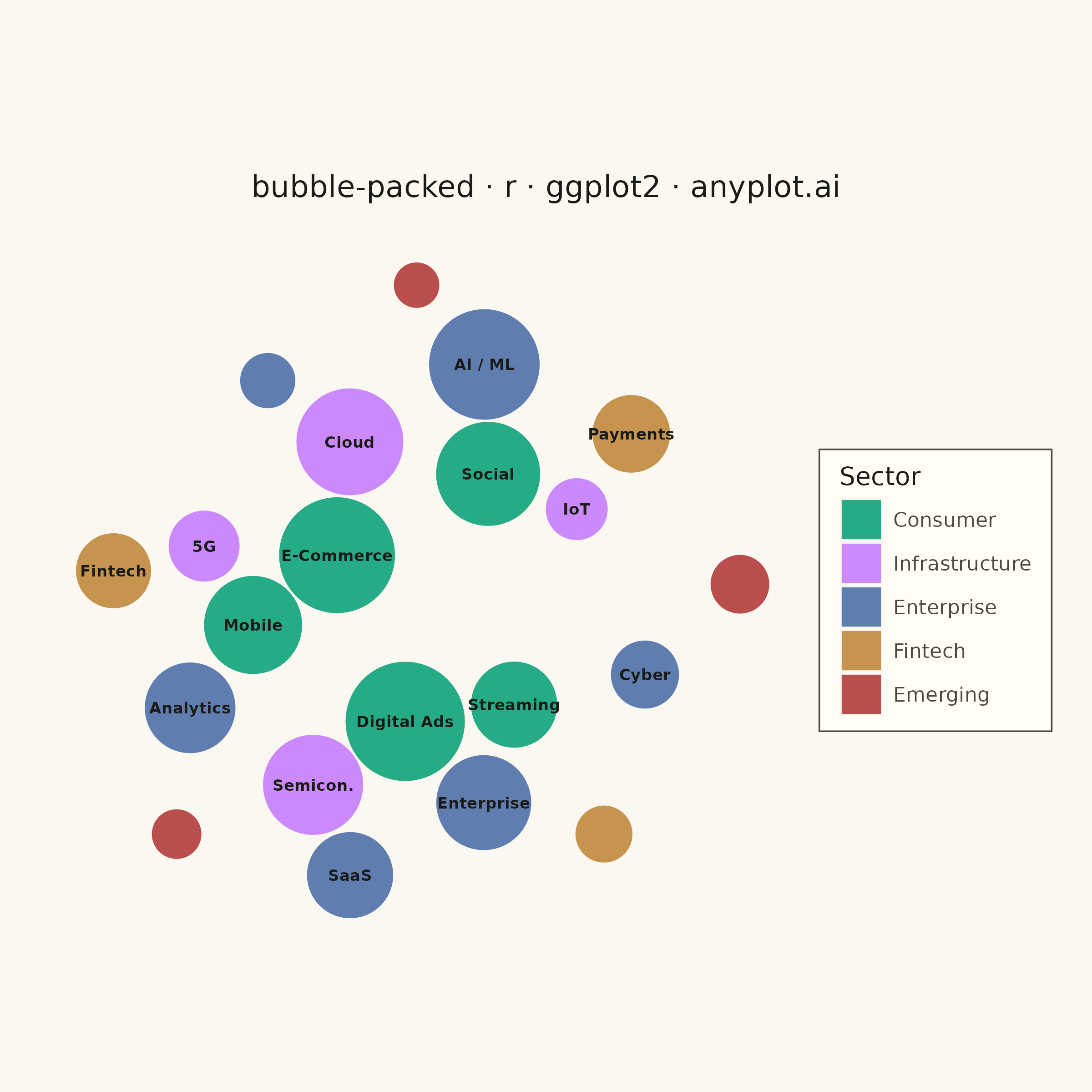
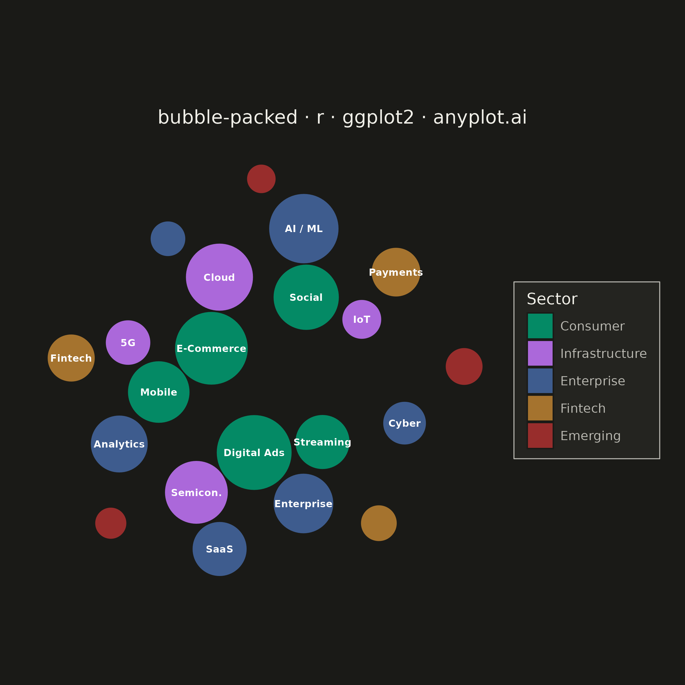
A packed bubble chart displays data as circles where size represents value, and circles are packed together without overlap using physics simulation. Unlike scatter or traditional bubble charts, position has no meaning - only size and optional grouping matter. This visualization efficiently uses space for comparing values across many categories.
#' anyplot.ai
#' bubble-packed: Basic Packed Bubble Chart
#' Library: ggplot2 3.5.1 | R 4.4.1
#' Quality: 86/100 | Created: 2026-05-29

library(ggplot2)
library(dplyr)
library(tibble)
library(ragg)

set.seed(42)

# Theme tokens — Imprint palette (see prompts/default-style-guide.md)
THEME       <- Sys.getenv("ANYPLOT_THEME", "light")
PAGE_BG     <- if (THEME == "light") "#FAF8F1" else "#1A1A17"
ELEVATED_BG <- if (THEME == "light") "#FFFDF6" else "#242420"
INK         <- if (THEME == "light") "#1A1A17" else "#F0EFE8"
INK_SOFT    <- if (THEME == "light") "#4A4A44" else "#B8B7B0"
LABEL_COLOR <- if (THEME == "light") INK else "#FFFFFF"

# Imprint categorical palette — first series always #009E73
IMPRINT_PALETTE <- c(
  "#009E73",  # 1 brand green  — Consumer
  "#C475FD",  # 2 lavender     — Infrastructure
  "#4467A3",  # 3 blue         — Enterprise
  "#BD8233",  # 4 ochre        — Fintech
  "#AE3030"   # 5 matte red    — Emerging
)

# Data: global technology market segments (estimated revenue $B)
sector_levels <- c("Consumer", "Infrastructure", "Enterprise", "Fintech", "Emerging")

segments <- tibble(
  label = c(
    "E-Commerce", "Digital Ads", "Social",     "Mobile",   "Streaming",
    "Cloud",      "Semicon.",    "IoT",        "5G",
    "Enterprise", "AI / ML",    "Analytics",  "Cyber",    "Dev Tools", "SaaS",
    "Payments",   "Fintech",    "InsurTech",
    "AR / VR",    "EdTech",     "HealthTech"
  ),
  value = c(
    680, 720, 550, 490, 380,
    580, 510, 200, 260,
    460, 620, 420, 240, 160, 380,
    310, 290, 170,
    110, 130, 180
  ),
  sector = c(
    "Consumer", "Consumer", "Consumer", "Consumer", "Consumer",
    "Infrastructure", "Infrastructure", "Infrastructure", "Infrastructure",
    "Enterprise", "Enterprise", "Enterprise", "Enterprise", "Enterprise", "Enterprise",
    "Fintech", "Fintech", "Fintech",
    "Emerging", "Emerging", "Emerging"
  )
) |>
  mutate(
    sector = factor(sector, levels = sector_levels),
    radius = sqrt(value) * 0.017  # area-proportional radii
  )

n_segs <- nrow(segments)

# Force-directed circle packing with sector clustering
pack_circles <- function(r, sectors = NULL, n_iter = 1500) {
  n  <- length(r)
  ga <- pi * (3 - sqrt(5))  # golden angle

  # Golden-angle spiral initial placement
  px <- numeric(n)
  py <- numeric(n)
  for (i in seq_len(n)) {
    ang   <- i * ga
    rs    <- sqrt(i) * mean(r) * 2.0
    px[i] <- rs * cos(ang)
    py[i] <- rs * sin(ang)
  }

  # Iterative overlap resolution with centroid + sector gravity
  for (it in seq_len(n_iter)) {
    any_mv <- FALSE
    for (i in seq_len(n - 1)) {
      for (j in (i + 1):n) {
        dx   <- px[i] - px[j]
        dy   <- py[i] - py[j]
        d    <- sqrt(dx * dx + dy * dy)
        dmin <- r[i] + r[j] + 2e-3

        if (d < dmin) {
          any_mv <- TRUE
          if (d < 1e-9) {
            px[j] <- px[j] + 1e-3 * runif(1, -1, 1)
            next
          }
          push   <- (dmin - d) * 0.51
          ux     <- dx / d
          uy     <- dy / d
          px[i]  <- px[i] + push * ux
          py[i]  <- py[i] + push * uy
          px[j]  <- px[j] - push * ux
          py[j]  <- py[j] - push * uy
        }
      }
    }

    # Global centroid gravity (tightens pack)
    g  <- 0.04
    cx <- mean(px)
    cy <- mean(py)
    px <- px + g * (cx - px)
    py <- py + g * (cy - py)

    # Sector centroid gravity (clusters same-sector circles)
    if (!is.null(sectors)) {
      gs <- 0.012
      for (s in unique(sectors)) {
        idx  <- which(sectors == s)
        scx  <- mean(px[idx])
        scy  <- mean(py[idx])
        px[idx] <- px[idx] + gs * (scx - px[idx])
        py[idx] <- py[idx] + gs * (scy - py[idx])
      }
    }

    if (!any_mv) break
  }

  # Final tightening: nudge each circle toward nearest non-overlapping neighbor
  for (pass in seq_len(8)) {
    for (i in seq_len(n)) {
      best_gap <- Inf
      best_j   <- NA_integer_
      for (j in seq_len(n)) {
        if (j == i) next
        d   <- sqrt((px[i] - px[j])^2 + (py[i] - py[j])^2)
        gap <- d - r[i] - r[j]
        if (gap > 0 && gap < best_gap) { best_gap <- gap; best_j <- j }
      }
      if (!is.na(best_j) && best_gap > 1e-3) {
        dx   <- px[best_j] - px[i]
        dy   <- py[best_j] - py[i]
        d    <- sqrt(dx^2 + dy^2)
        step <- min(best_gap * 0.45, 0.04)
        px[i] <- px[i] + step * dx / d
        py[i] <- py[i] + step * dy / d
      }
    }
    # Re-resolve any overlaps introduced by tightening
    for (i in seq_len(n - 1)) {
      for (j in (i + 1):n) {
        dx   <- px[i] - px[j]; dy <- py[i] - py[j]
        d    <- sqrt(dx^2 + dy^2); dmin <- r[i] + r[j] + 2e-3
        if (d < dmin && d > 1e-9) {
          push  <- (dmin - d) * 0.51; ux <- dx / d; uy <- dy / d
          px[i] <- px[i] + push * ux; py[i] <- py[i] + push * uy
          px[j] <- px[j] - push * ux; py[j] <- py[j] - push * uy
        }
      }
    }
  }

  list(x = px - mean(px), y = py - mean(py))
}

pos      <- pack_circles(segments$radius, sectors = as.character(segments$sector))
segments <- segments |> mutate(x = pos$x, y = pos$y)

# Circle polygons for geom_polygon
n_pts        <- 72
circle_polys <- bind_rows(lapply(seq_len(n_segs), function(i) {
  s     <- segments[i, ]
  theta <- seq(0, 2 * pi, length.out = n_pts + 1)
  tibble(
    x      = s$x + s$radius * cos(theta),
    y      = s$y + s$radius * sin(theta),
    id     = i,
    sector = as.character(s$sector)
  )
})) |>
  mutate(sector = factor(sector, levels = sector_levels))

# Labels only for circles large enough to hold text
label_df <- segments |> filter(radius >= 0.24)

# Title — square canvas, no scaling needed (42 chars < 67)
plot_title <- "bubble-packed · r · ggplot2 · anyplot.ai"
n_chr      <- nchar(plot_title)
title_sz   <- if (n_chr > 67) round(12 * 67 / n_chr) else 12

p <- ggplot() +
  geom_polygon(
    data      = circle_polys,
    aes(x = x, y = y, group = id, fill = sector),
    alpha     = 0.85,
    color     = PAGE_BG,
    linewidth = 0.35
  ) +
  geom_text(
    data     = label_df,
    aes(x = x, y = y, label = label),
    color    = LABEL_COLOR,
    size     = 2.2,
    fontface = "bold"
  ) +
  scale_fill_manual(
    values = setNames(IMPRINT_PALETTE, sector_levels),
    name   = "Sector"
  ) +
  coord_equal() +
  labs(title = plot_title) +
  theme_void(base_size = 8) +
  theme(
    plot.background   = element_rect(fill = PAGE_BG,     color = NA),
    panel.background  = element_rect(fill = PAGE_BG,     color = NA),
    plot.title          = element_text(
      color  = INK,
      size   = title_sz,
      hjust  = 0.5,
      face   = "plain",
      margin = margin(t = 14, b = 10)
    ),
    plot.title.position = "plot",
    legend.position   = "right",
    legend.text       = element_text(color = INK_SOFT, size = 8),
    legend.title      = element_text(color = INK,      size = 10),
    legend.background = element_rect(fill = ELEVATED_BG, color = INK_SOFT, linewidth = 0.3),
    legend.margin     = margin(6, 8, 6, 8),
    plot.margin       = margin(16, 16, 16, 16)
  )

# Save — square canvas: 6 x 6 in @ 400 dpi = 2400 x 2400 px
ggsave(
  filename = sprintf("plot-%s.png", THEME),
  plot     = p,
  device   = ragg::agg_png,
  width    = 6,
  height   = 6,
  units    = "in",
  dpi      = 400
)
Runnable source as JSON, for any HTTP client: https://api.anyplot.ai/specs/bubble-packed/ggplot2/code. Any spec id and library id listed in llms-full.txt fit the same URL shape; every URL below is complete and callable.
{
  "spec_id": "bubble-packed",
  "language": "r",
  "library": "ggplot2",
  "page": "https://anyplot.ai/bubble-packed/r/ggplot2",
  "hub": "https://anyplot.ai/bubble-packed",
  "code_json": "https://api.anyplot.ai/specs/bubble-packed/ggplot2/code",
  "spec_json": "https://api.anyplot.ai/specs/bubble-packed",
  "render_light_png": "https://storage.googleapis.com/anyplot-images/plots/bubble-packed/r/ggplot2/plot-light.png",
  "render_dark_png": "https://storage.googleapis.com/anyplot-images/plots/bubble-packed/r/ggplot2/plot-dark.png",
  "quality_score": 86.0,
  "license": "MIT",
  "guide": "https://anyplot.ai/llms.txt"
}
Part of Basic Packed Bubble Chart on anyplot.ai.