The same plot in 14 other libraries — JavaScript: Chart.js, Apache ECharts, Highcharts, MUI X Charts; Python: Altair, Bokeh, lets-plot, Matplotlib, Plotly, plotnine, Pygal, Seaborn; R: ggplot2; Julia: Makie.jl. Compare all 15 side by side: Cartogram with Area Distortion by Data Value in Python, R, Julia and JavaScript.
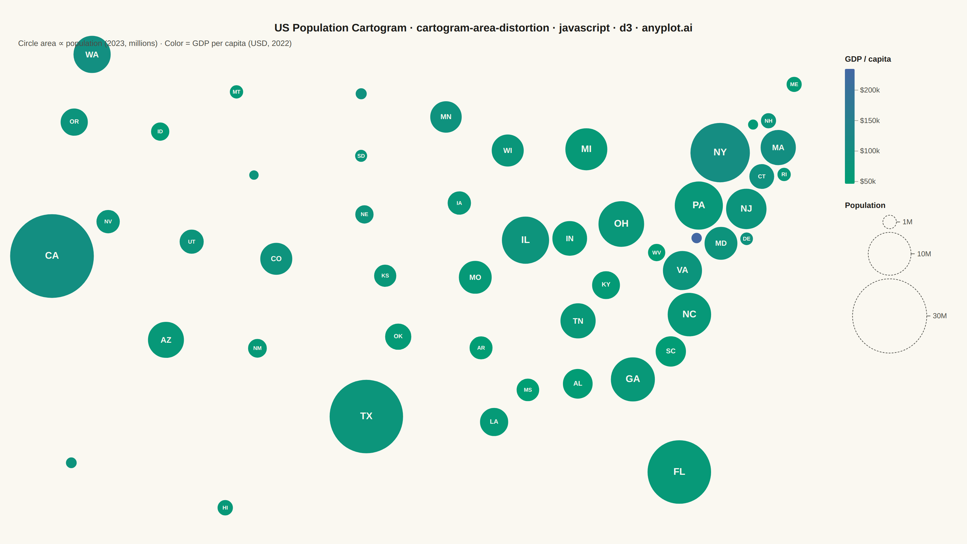
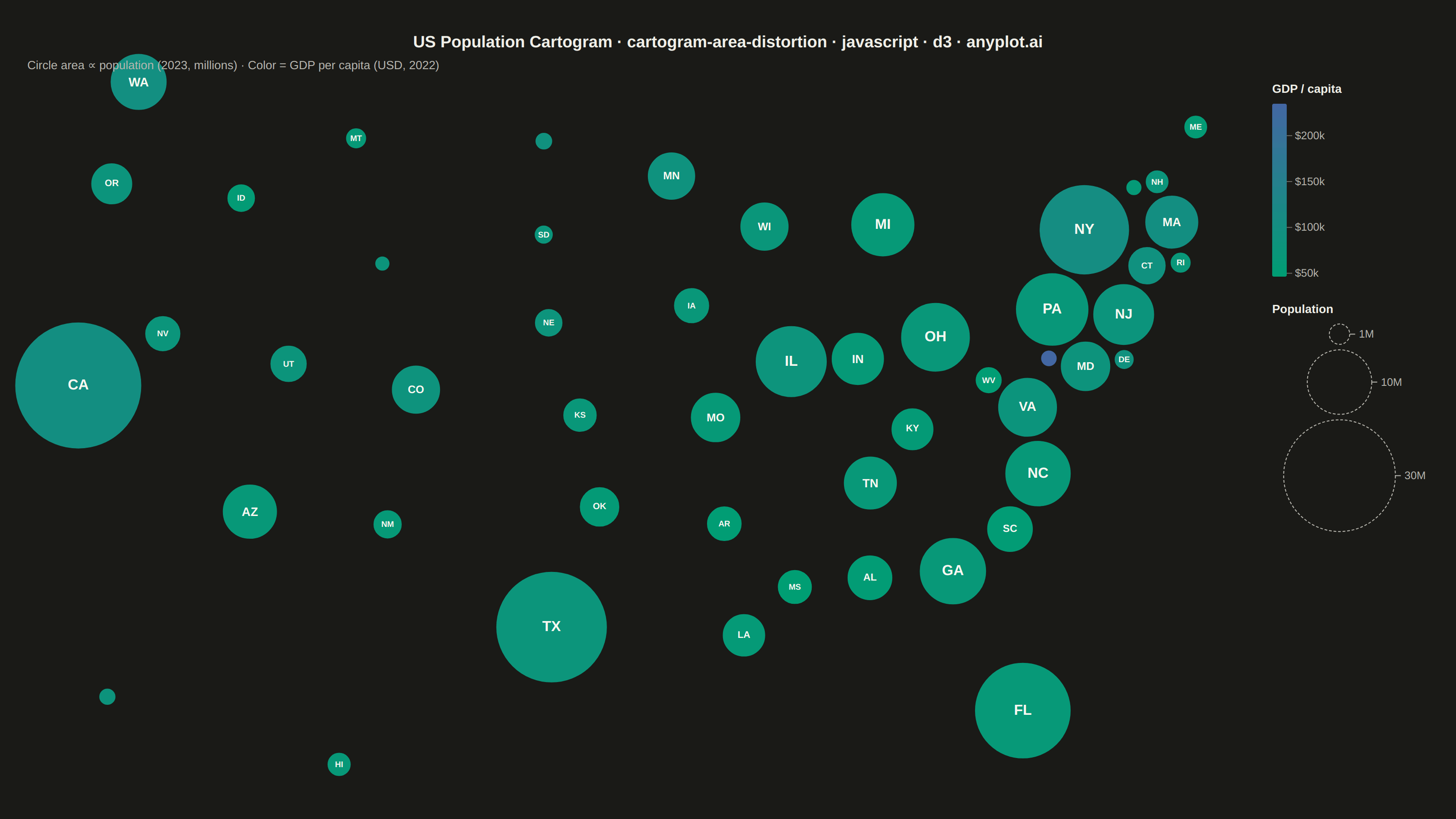
A cartogram distorts geographic regions so that their area becomes proportional to a data variable (e.g., population, GDP, election votes) rather than physical land area. This solves the classic problem of large but sparsely populated areas dominating standard maps, making it easier to compare values across regions at a glance. Contiguous cartograms preserve adjacency and rough shape of regions while rescaling them, famously used in election coverage worldwide.
// anyplot.ai
// cartogram-area-distortion: Cartogram with Area Distortion by Data Value
// Library: d3 7.9.0 | JavaScript 22.22.3
// Quality: 84/100 | Created: 2026-06-08

const t = window.ANYPLOT_TOKENS;
const { width, height } = window.ANYPLOT_SIZE;

const margin = { top: 130, right: 230, bottom: 60, left: 30 };
const iw = width - margin.left - margin.right;
const ih = height - margin.top - margin.bottom;

// US states: name, abbreviation, centroid lon/lat, population 2023 (M), GDP 2022 (B$)
const states = [
  { name: "Alabama",        abbr: "AL", lon: -86.7,  lat: 32.8, pop: 5.1,  gdp: 271  },
  { name: "Alaska",         abbr: "AK", lon: -153.0, lat: 64.2, pop: 0.74, gdp: 61   },
  { name: "Arizona",        abbr: "AZ", lon: -111.7, lat: 34.3, pop: 7.4,  gdp: 488  },
  { name: "Arkansas",       abbr: "AR", lon: -92.4,  lat: 34.9, pop: 3.1,  gdp: 155  },
  { name: "California",     abbr: "CA", lon: -119.7, lat: 37.2, pop: 39.0, gdp: 3890 },
  { name: "Colorado",       abbr: "CO", lon: -105.5, lat: 39.0, pop: 5.9,  gdp: 498  },
  { name: "Connecticut",    abbr: "CT", lon: -72.7,  lat: 41.6, pop: 3.6,  gdp: 331  },
  { name: "Delaware",       abbr: "DE", lon: -75.5,  lat: 39.0, pop: 1.0,  gdp: 91   },
  { name: "Florida",        abbr: "FL", lon: -81.5,  lat: 27.8, pop: 22.6, gdp: 1460 },
  { name: "Georgia",        abbr: "GA", lon: -83.4,  lat: 32.7, pop: 11.0, gdp: 743  },
  { name: "Hawaii",         abbr: "HI", lon: -157.5, lat: 20.3, pop: 1.44, gdp: 96   },
  { name: "Idaho",          abbr: "ID", lon: -114.5, lat: 44.4, pop: 2.0,  gdp: 110  },
  { name: "Illinois",       abbr: "IL", lon: -89.2,  lat: 40.1, pop: 12.6, gdp: 1023 },
  { name: "Indiana",        abbr: "IN", lon: -86.3,  lat: 40.0, pop: 6.9,  gdp: 432  },
  { name: "Iowa",           abbr: "IA", lon: -93.5,  lat: 42.1, pop: 3.2,  gdp: 229  },
  { name: "Kansas",         abbr: "KS", lon: -98.4,  lat: 38.5, pop: 2.9,  gdp: 207  },
  { name: "Kentucky",       abbr: "KY", lon: -84.3,  lat: 37.5, pop: 4.5,  gdp: 263  },
  { name: "Louisiana",      abbr: "LA", lon: -91.8,  lat: 31.2, pop: 4.6,  gdp: 279  },
  { name: "Maine",          abbr: "ME", lon: -69.2,  lat: 45.4, pop: 1.4,  gdp: 79   },
  { name: "Maryland",       abbr: "MD", lon: -76.8,  lat: 39.1, pop: 6.2,  gdp: 511  },
  { name: "Massachusetts",  abbr: "MA", lon: -71.8,  lat: 42.3, pop: 7.1,  gdp: 709  },
  { name: "Michigan",       abbr: "MI", lon: -84.5,  lat: 44.3, pop: 10.0, gdp: 634  },
  { name: "Minnesota",      abbr: "MN", lon: -94.3,  lat: 46.4, pop: 5.7,  gdp: 501  },
  { name: "Mississippi",    abbr: "MS", lon: -89.7,  lat: 32.7, pop: 3.0,  gdp: 139  },
  { name: "Missouri",       abbr: "MO", lon: -92.6,  lat: 38.4, pop: 6.2,  gdp: 395  },
  { name: "Montana",        abbr: "MT", lon: -109.6, lat: 47.0, pop: 1.1,  gdp: 68   },
  { name: "Nebraska",       abbr: "NE", lon: -99.9,  lat: 41.5, pop: 2.0,  gdp: 163  },
  { name: "Nevada",         abbr: "NV", lon: -116.7, lat: 39.5, pop: 3.2,  gdp: 244  },
  { name: "New Hampshire",  abbr: "NH", lon: -71.6,  lat: 43.7, pop: 1.4,  gdp: 109  },
  { name: "New Jersey",     abbr: "NJ", lon: -74.5,  lat: 40.1, pop: 9.3,  gdp: 748  },
  { name: "New Mexico",     abbr: "NM", lon: -106.1, lat: 34.5, pop: 2.1,  gdp: 131  },
  { name: "New York",       abbr: "NY", lon: -75.5,  lat: 42.9, pop: 19.8, gdp: 2053 },
  { name: "North Carolina", abbr: "NC", lon: -79.4,  lat: 35.6, pop: 10.7, gdp: 714  },
  { name: "North Dakota",   abbr: "ND", lon: -100.5, lat: 47.5, pop: 0.78, gdp: 71   },
  { name: "Ohio",           abbr: "OH", lon: -82.8,  lat: 40.4, pop: 11.8, gdp: 838  },
  { name: "Oklahoma",       abbr: "OK", lon: -97.5,  lat: 35.5, pop: 4.0,  gdp: 239  },
  { name: "Oregon",         abbr: "OR", lon: -120.5, lat: 43.9, pop: 4.3,  gdp: 347  },
  { name: "Pennsylvania",   abbr: "PA", lon: -77.2,  lat: 40.6, pop: 13.1, gdp: 913  },
  { name: "Rhode Island",   abbr: "RI", lon: -71.5,  lat: 41.7, pop: 1.1,  gdp: 79   },
  { name: "South Carolina", abbr: "SC", lon: -80.9,  lat: 33.8, pop: 5.3,  gdp: 281  },
  { name: "South Dakota",   abbr: "SD", lon: -100.3, lat: 44.4, pop: 0.91, gdp: 71   },
  { name: "Tennessee",      abbr: "TN", lon: -86.3,  lat: 35.9, pop: 7.1,  gdp: 481  },
  { name: "Texas",          abbr: "TX", lon: -99.3,  lat: 31.5, pop: 30.1, gdp: 2355 },
  { name: "Utah",           abbr: "UT", lon: -111.1, lat: 39.3, pop: 3.4,  gdp: 270  },
  { name: "Vermont",        abbr: "VT", lon: -72.7,  lat: 44.0, pop: 0.65, gdp: 40   },
  { name: "Virginia",       abbr: "VA", lon: -79.4,  lat: 37.5, pop: 8.7,  gdp: 704  },
  { name: "Washington",     abbr: "WA", lon: -120.5, lat: 47.4, pop: 7.9,  gdp: 785  },
  { name: "West Virginia",  abbr: "WV", lon: -80.6,  lat: 38.6, pop: 1.8,  gdp: 89   },
  { name: "Wisconsin",      abbr: "WI", lon: -90.0,  lat: 44.6, pop: 5.9,  gdp: 433  },
  { name: "Wyoming",        abbr: "WY", lon: -107.6, lat: 43.0, pop: 0.58, gdp: 46   },
  { name: "D.C.",           abbr: "DC", lon: -77.0,  lat: 38.9, pop: 0.69, gdp: 162  },
];

// GDP per capita in USD
states.forEach(d => { d.gdpPerCapita = (d.gdp / d.pop) * 1000; });

// AlbersUSA composite projection handles AK + HI insets automatically
const geoFeatures = {
  type: "FeatureCollection",
  features: states.map(d => ({
    type: "Feature",
    geometry: { type: "Point", coordinates: [d.lon, d.lat] },
  })),
};

const projection = d3.geoAlbersUsa().fitExtent(
  [[0, 12], [iw, ih]],
  geoFeatures
);

states.forEach(d => {
  const p = projection([d.lon, d.lat]);
  d.x = p ? p[0] : iw / 2;
  d.y = p ? p[1] : ih / 2;
});

// Radius scale: area ∝ population (Dorling cartogram style)
const maxPop = d3.max(states, d => d.pop);
const maxR = 70;
const rScale = d3.scaleSqrt().domain([0, maxPop]).range([0, maxR]);

// Save projected positions as attraction anchors
states.forEach(d => { d.x0 = d.x; d.y0 = d.y; });

// Force simulation: pull circles toward geographic centroids, repel overlaps
const sim = d3.forceSimulation(states)
  .force("attract-x", d3.forceX(d => d.x0).strength(0.65))
  .force("attract-y", d3.forceY(d => d.y0).strength(0.65))
  .force("collide", d3.forceCollide(d => rScale(d.pop) + 2).strength(1.0))
  .stop();

for (let i = 0; i < 350; i++) sim.tick();

// Color: GDP per capita using Imprint sequential scale (green → blue)
const gdpPCValues = states.map(d => d.gdpPerCapita);
const minGdpPC = d3.min(gdpPCValues);
const maxGdpPC = d3.max(gdpPCValues);
const colorScale = d3.scaleSequential(
  d3.interpolateRgbBasis(t.seq)
).domain([minGdpPC, maxGdpPC]);

// SVG
const svg = d3.select("#container")
  .append("svg")
  .attr("width", width)
  .attr("height", height);

const g = svg.append("g")
  .attr("transform", `translate(${margin.left},${margin.top})`);

// Circles — sorted by size descending so small circles render on top
const sortedStates = [...states].sort((a, b) => b.pop - a.pop);

g.selectAll("circle.state")
  .data(sortedStates)
  .join("circle")
  .attr("class", "state")
  .attr("cx", d => d.x)
  .attr("cy", d => d.y)
  .attr("r", d => rScale(d.pop))
  .attr("fill", d => colorScale(d.gdpPerCapita))
  .attr("stroke", t.pageBg)
  .attr("stroke-width", 1.5);

// Abbreviation labels: threshold lowered to 8px; AK always labeled
g.selectAll("text.abbr")
  .data(states.filter(d => rScale(d.pop) >= 8 || d.abbr === "AK"))
  .join("text")
  .attr("class", "abbr")
  .attr("x", d => d.x)
  .attr("y", d => d.y)
  .attr("text-anchor", "middle")
  .attr("dominant-baseline", "central")
  .attr("fill", t.pageBg)
  .style("font-size", d => `${Math.max(9, Math.min(16, rScale(d.pop) * 0.44))}px`)
  .style("font-weight", "700")
  .style("pointer-events", "none")
  .text(d => d.abbr);

// --- Geographic reference inset (bottom-right of inner plot) ---
// Shows states at equal size by actual geographic position — contrast with cartogram
const insetW = 270, insetH = 155;
const insetX = iw - insetW - 4;
const insetY = ih - insetH - 4;

const insetProj = d3.geoAlbersUsa().fitExtent(
  [[6, 6], [insetW - 6, insetH - 22]],
  geoFeatures
);

g.append("rect")
  .attr("x", insetX)
  .attr("y", insetY)
  .attr("width", insetW)
  .attr("height", insetH)
  .attr("fill", t.elevatedBg)
  .attr("stroke", t.grid)
  .attr("stroke-width", 1)
  .attr("rx", 4)
  .attr("opacity", 0.95);

g.append("text")
  .attr("x", insetX + insetW / 2)
  .attr("y", insetY + insetH - 5)
  .attr("text-anchor", "middle")
  .attr("fill", t.inkSoft)
  .style("font-size", "13px")
  .style("font-style", "italic")
  .text("Geographic reference (equal-size dots)");

states.forEach(d => {
  const p = insetProj([d.lon, d.lat]);
  if (!p) return;
  g.append("circle")
    .attr("cx", insetX + p[0])
    .attr("cy", insetY + p[1])
    .attr("r", 4)
    .attr("fill", colorScale(d.gdpPerCapita))
    .attr("stroke", t.pageBg)
    .attr("stroke-width", 0.8);
});

// Title (scaled for length)
const titleStr = "US Population Cartogram · cartogram-area-distortion · javascript · d3 · anyplot.ai";
const titlePx = Math.round(22 * Math.min(1, 67 / titleStr.length));

svg.append("text")
  .attr("x", width / 2)
  .attr("y", 52)
  .attr("text-anchor", "middle")
  .attr("fill", t.ink)
  .style("font-size", `${titlePx}px`)
  .style("font-weight", "600")
  .text(titleStr);

// Subtitle — moved to y=96 to clear WA circle overlap; font bumped to 14px
svg.append("text")
  .attr("x", margin.left)
  .attr("y", 96)
  .attr("fill", t.inkSoft)
  .style("font-size", "14px")
  .text("Circle area ∝ population (2023, millions) · Color = GDP per capita (USD, 2022)");

// --- Color legend ---
const legX = margin.left + iw + 28;
const legY = margin.top + 24;
const legH = 190;
const legW = 16;

const defs = svg.append("defs");
const grad = defs.append("linearGradient")
  .attr("id", "cleg-grad")
  .attr("x1", "0%").attr("y1", "100%")
  .attr("x2", "0%").attr("y2", "0%");

[0, 0.25, 0.5, 0.75, 1].forEach(s => {
  grad.append("stop")
    .attr("offset", `${s * 100}%`)
    .attr("stop-color", colorScale(minGdpPC + s * (maxGdpPC - minGdpPC)));
});

svg.append("rect")
  .attr("x", legX)
  .attr("y", legY)
  .attr("width", legW)
  .attr("height", legH)
  .attr("fill", "url(#cleg-grad)")
  .attr("rx", 2);

const cLegScale = d3.scaleLinear().domain([minGdpPC, maxGdpPC]).range([legH, 0]);
const cAxis = d3.axisRight(cLegScale)
  .ticks(5)
  .tickFormat(d => `$${Math.round(d / 1000)}k`);

const cAxisG = svg.append("g")
  .attr("transform", `translate(${legX + legW}, ${legY})`)
  .call(cAxis);

cAxisG.selectAll("text").attr("fill", t.inkSoft).style("font-size", "13px");
cAxisG.selectAll("line").attr("stroke", t.inkSoft).attr("stroke-opacity", 0.5);
cAxisG.select(".domain").remove();

svg.append("text")
  .attr("x", legX)
  .attr("y", legY - 12)
  .attr("fill", t.ink)
  .style("font-size", "14px")
  .style("font-weight", "600")
  .text("GDP / capita");

// --- Size legend ---
const szLegY = legY + legH + 52;

svg.append("text")
  .attr("x", legX)
  .attr("y", szLegY - 12)
  .attr("fill", t.ink)
  .style("font-size", "14px")
  .style("font-weight", "600")
  .text("Population");

const szVals = [1, 10, 30];
const szCx = legX + maxR + 4;
let szY = szLegY;

szVals.forEach(v => {
  const r = rScale(v);
  szY += r;
  svg.append("circle")
    .attr("cx", szCx)
    .attr("cy", szY)
    .attr("r", r)
    .attr("fill", "none")
    .attr("stroke", t.inkSoft)
    .attr("stroke-width", 1)
    .attr("stroke-dasharray", "3,2");
  svg.append("line")
    .attr("x1", szCx + r)
    .attr("y1", szY)
    .attr("x2", szCx + r + 6)
    .attr("y2", szY)
    .attr("stroke", t.inkSoft)
    .attr("stroke-width", 1);
  svg.append("text")
    .attr("x", szCx + r + 10)
    .attr("y", szY + 4)
    .attr("fill", t.inkSoft)
    .style("font-size", "13px")
    .text(`${v}M`);
  szY += r + 6;
});
Runnable source as JSON, for any HTTP client: https://api.anyplot.ai/specs/cartogram-area-distortion/d3/code. Any spec id and library id listed in llms-full.txt fit the same URL shape; every URL below is complete and callable.
{
  "spec_id": "cartogram-area-distortion",
  "language": "javascript",
  "library": "d3",
  "page": "https://anyplot.ai/cartogram-area-distortion/javascript/d3",
  "hub": "https://anyplot.ai/cartogram-area-distortion",
  "code_json": "https://api.anyplot.ai/specs/cartogram-area-distortion/d3/code",
  "spec_json": "https://api.anyplot.ai/specs/cartogram-area-distortion",
  "render_light_png": "https://storage.googleapis.com/anyplot-images/plots/cartogram-area-distortion/javascript/d3/plot-light.png",
  "render_dark_png": "https://storage.googleapis.com/anyplot-images/plots/cartogram-area-distortion/javascript/d3/plot-dark.png",
  "interactive_light_html": "https://storage.googleapis.com/anyplot-images/plots/cartogram-area-distortion/javascript/d3/plot-light.html",
  "interactive_dark_html": "https://storage.googleapis.com/anyplot-images/plots/cartogram-area-distortion/javascript/d3/plot-dark.html",
  "quality_score": 84.0,
  "license": "MIT",
  "guide": "https://anyplot.ai/llms.txt"
}
Part of Cartogram with Area Distortion by Data Value on anyplot.ai.