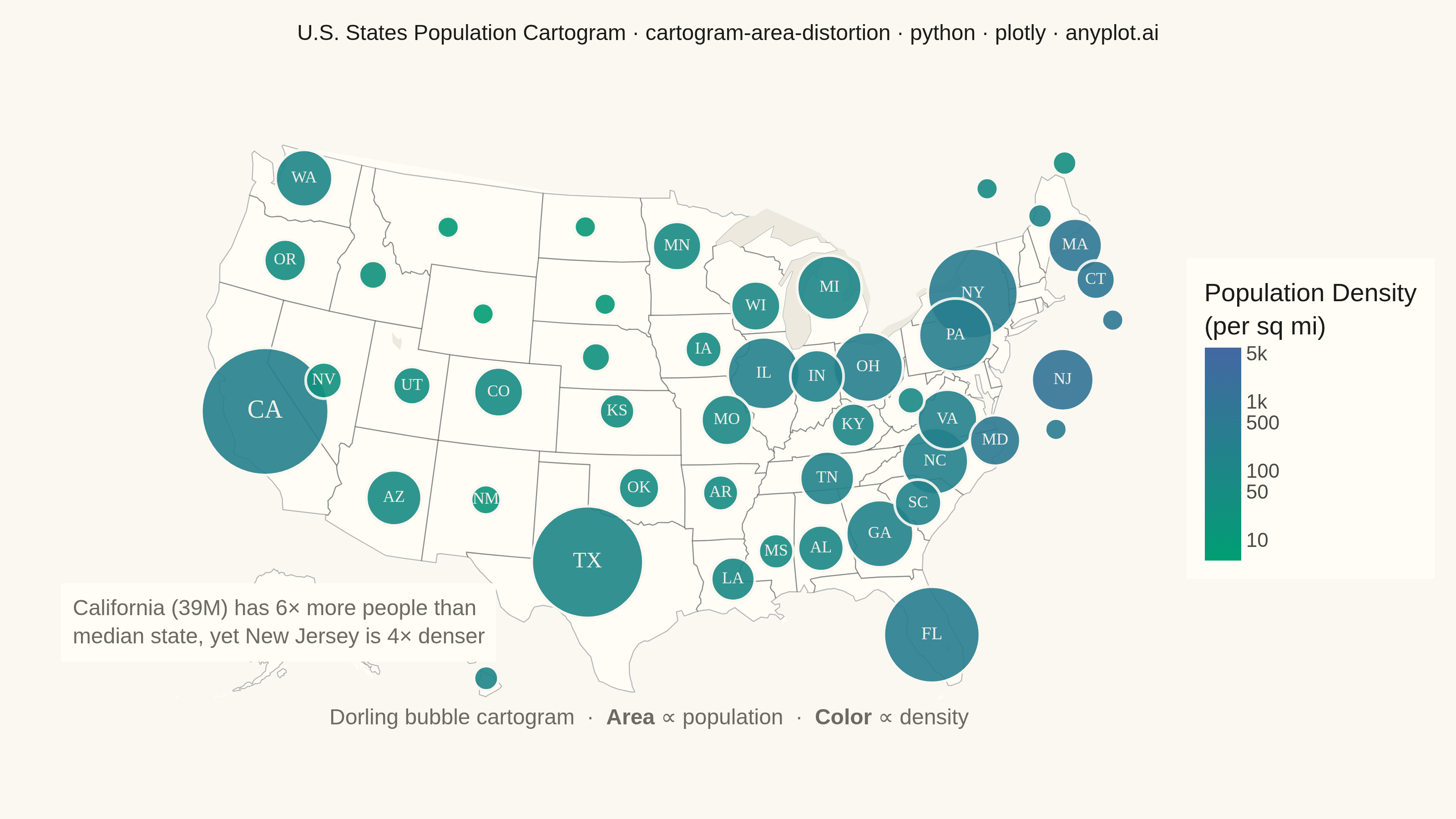
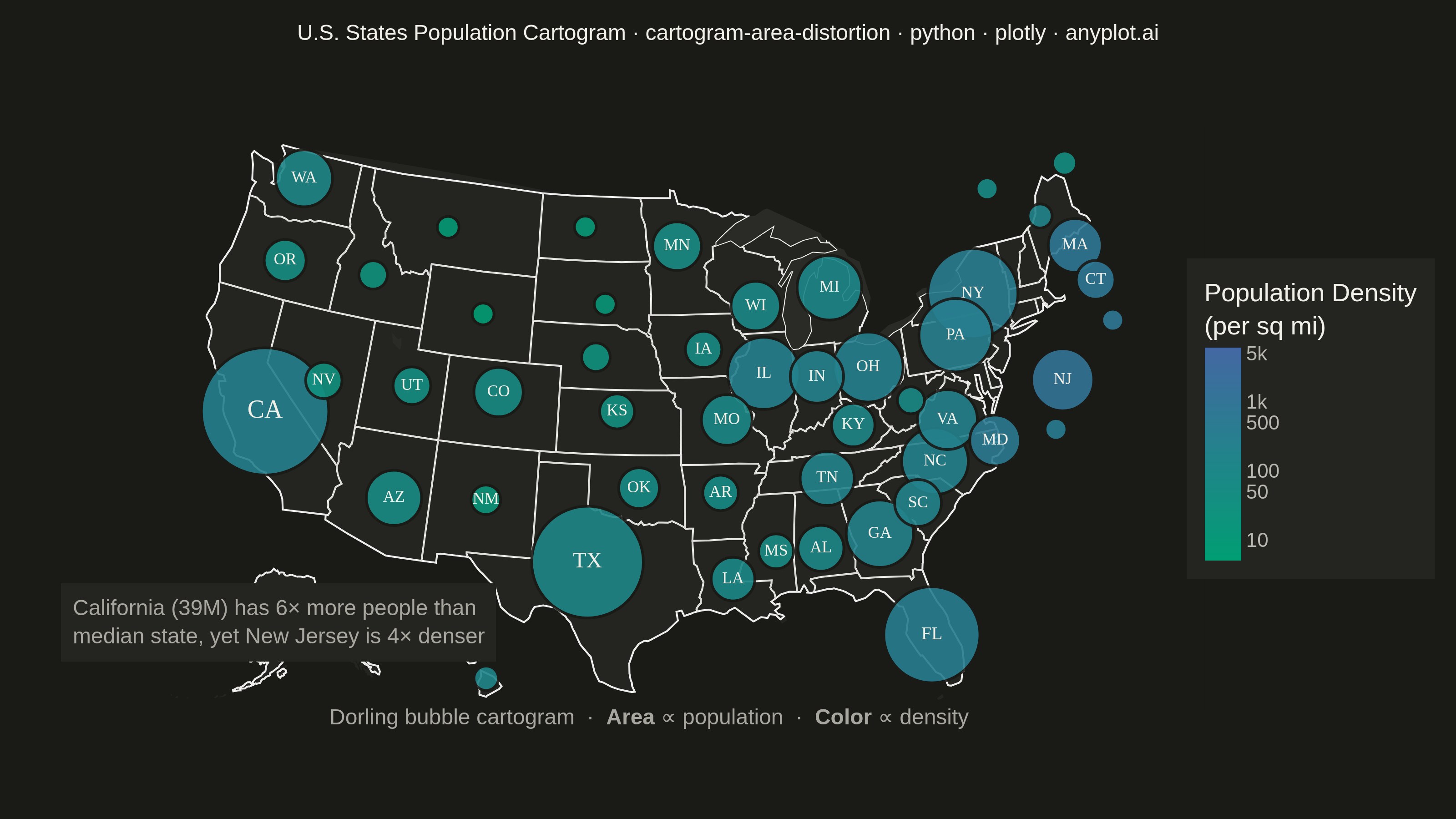
A cartogram distorts geographic regions so that their area becomes proportional to a data variable (e.g., population, GDP, election votes) rather than physical land area. This solves the classic problem of large but sparsely populated areas dominating standard maps, making it easier to compare values across regions at a glance. Contiguous cartograms preserve adjacency and rough shape of regions while rescaling them, famously used in election coverage worldwide.
""" anyplot.ai
cartogram-area-distortion: Cartogram with Area Distortion by Data Value
Library: plotly 6.8.0 | Python 3.13.13
Quality: 82/100 | Updated: 2026-06-08
"""

import os

import numpy as np
import plotly.graph_objects as go


# Theme tokens (Imprint palette, theme-adaptive chrome)
THEME = os.getenv("ANYPLOT_THEME", "light")
PAGE_BG = "#FAF8F1" if THEME == "light" else "#1A1A17"
ELEVATED_BG = "#FFFDF6" if THEME == "light" else "#242420"
INK = "#1A1A17" if THEME == "light" else "#F0EFE8"
INK_SOFT = "#4A4A44" if THEME == "light" else "#B8B7B0"
INK_MUTED = "#6B6A63" if THEME == "light" else "#A8A79F"

# Imprint sequential colorscale for continuous density data
imprint_seq = [[0.0, "#009E73"], [1.0, "#4467A3"]]

# Data - US states sized by population (2023 Census estimates, millions)
states = [
    "CA",
    "TX",
    "FL",
    "NY",
    "PA",
    "IL",
    "OH",
    "GA",
    "NC",
    "MI",
    "NJ",
    "VA",
    "WA",
    "AZ",
    "MA",
    "TN",
    "IN",
    "MO",
    "MD",
    "WI",
    "CO",
    "MN",
    "SC",
    "AL",
    "LA",
    "KY",
    "OR",
    "OK",
    "CT",
    "UT",
    "IA",
    "NV",
    "AR",
    "MS",
    "KS",
    "NM",
    "NE",
    "ID",
    "WV",
    "HI",
    "NH",
    "ME",
    "MT",
    "RI",
    "DE",
    "SD",
    "ND",
    "AK",
    "VT",
    "WY",
]

population = np.array(
    [
        39.03,
        30.03,
        22.24,
        19.57,
        12.97,
        12.55,
        11.78,
        10.91,
        10.70,
        10.04,
        9.29,
        8.64,
        7.81,
        7.36,
        7.00,
        7.05,
        6.83,
        6.18,
        6.18,
        5.89,
        5.84,
        5.71,
        5.28,
        5.07,
        4.59,
        4.53,
        4.24,
        4.00,
        3.62,
        3.42,
        3.20,
        3.18,
        3.05,
        2.94,
        2.94,
        2.11,
        1.97,
        1.94,
        1.77,
        1.44,
        1.40,
        1.39,
        1.12,
        1.10,
        1.02,
        0.91,
        0.78,
        0.74,
        0.65,
        0.58,
    ]
)

area_sq_miles = np.array(
    [
        163696,
        268596,
        65758,
        54555,
        46054,
        57914,
        44826,
        59425,
        53819,
        96714,
        8723,
        42775,
        71298,
        113990,
        10554,
        42144,
        36420,
        69707,
        12406,
        65496,
        104094,
        86936,
        32020,
        52420,
        52378,
        40408,
        98379,
        69899,
        5543,
        84897,
        56273,
        110572,
        53179,
        48432,
        82278,
        121590,
        77348,
        83569,
        24230,
        10932,
        9349,
        35380,
        147040,
        1545,
        2489,
        77116,
        70698,
        665384,
        9616,
        97813,
    ]
)

lats = np.array(
    [
        36.78,
        31.97,
        27.66,
        42.93,
        41.20,
        40.63,
        40.42,
        32.68,
        35.63,
        44.31,
        40.06,
        37.43,
        47.75,
        34.05,
        42.41,
        35.52,
        40.27,
        38.57,
        39.05,
        43.78,
        39.55,
        46.73,
        33.84,
        32.32,
        31.17,
        37.84,
        43.80,
        35.47,
        41.60,
        39.32,
        41.88,
        38.80,
        35.20,
        32.35,
        39.01,
        34.52,
        41.49,
        44.07,
        38.60,
        19.90,
        43.19,
        45.25,
        46.88,
        41.58,
        38.91,
        43.97,
        47.55,
        63.59,
        44.56,
        43.08,
    ]
)

lons = np.array(
    [
        -119.42,
        -99.90,
        -81.52,
        -75.58,
        -77.19,
        -89.40,
        -82.91,
        -83.54,
        -79.81,
        -84.71,
        -74.41,
        -78.66,
        -120.74,
        -111.09,
        -71.38,
        -86.15,
        -86.13,
        -91.83,
        -76.64,
        -89.62,
        -105.78,
        -94.69,
        -81.16,
        -86.90,
        -91.87,
        -84.27,
        -120.55,
        -97.09,
        -72.76,
        -111.09,
        -93.10,
        -116.42,
        -92.37,
        -89.40,
        -98.48,
        -105.87,
        -99.90,
        -114.74,
        -80.62,
        -155.58,
        -71.57,
        -69.45,
        -110.36,
        -71.48,
        -75.53,
        -99.44,
        -101.00,
        -154.49,
        -72.58,
        -107.29,
    ]
)

density = population * 1e6 / area_sq_miles

# NE state offsets fan states into distinct positions to avoid bubble overlap
ne_offsets = {
    "NJ": (-2.0, 3.0),  # → (38.1, -71.4) over Atlantic SE of NJ
    "CT": (0.5, 5.0),  # → (42.1, -67.8) east of Maine coast
    "MA": (1.5, 3.0),  # → (43.9, -68.4) NE of natural position
    "RI": (-1.5, 4.0),  # → (40.1, -67.5) well east of CT
    "NH": (2.5, 1.5),  # → (45.7, -70.1) north-east
    "VT": (3.0, -0.5),  # → (47.6, -73.1) far north
    "DE": (-3.0, 3.0),  # → (35.9, -72.5) far south over Atlantic
    "MD": (-3.0, 0.5),  # → (36.1, -76.1) far south
    "ME": (2.5, 2.0),  # → (47.8, -67.5) far north-east
}
for i, s in enumerate(states):
    if s in ne_offsets:
        dlat, dlon = ne_offsets[s]
        lats[i] += dlat
        lons[i] += dlon

# Scale bubble sizes: area proportional to population
max_marker_size = 70
raw_sizes = np.sqrt(population / population.max()) * max_marker_size
sizes = np.clip(raw_sizes, 12, max_marker_size)

# Log scale for density color mapping
log_density = np.log10(density)

# Labels for states >= 2M population
label_texts = [s if p >= 2.0 else "" for s, p in zip(states, population, strict=False)]

# Title — mandatory format; scale fontsize to prevent overflow at this length
title_str = "U.S. States Population Cartogram · cartogram-area-distortion · python · plotly · anyplot.ai"
title_fontsize = max(11, round(16 * 67 / len(title_str)))

# Theme-adaptive geo background colors
land_color = "#FFFDF6" if THEME == "light" else "#242420"
lake_color = "#EDE9DF" if THEME == "light" else "#2A2A26"
boundary_color = "rgba(74,74,68,0.4)" if THEME == "light" else "rgba(184,183,176,0.3)"

fig = go.Figure()

# Reference layer: faint state boundary outlines for geographic context
fig.add_trace(
    go.Choropleth(
        locationmode="USA-states",
        locations=states,
        z=[0] * len(states),
        colorscale=[[0, "rgba(0,0,0,0)"], [1, "rgba(0,0,0,0)"]],
        showscale=False,
        marker={"line": {"color": boundary_color, "width": 0.6}},
        hoverinfo="skip",
    )
)

# Bubble cartogram: size ∝ population, color ∝ density (Imprint sequential)
fig.add_trace(
    go.Scattergeo(
        locationmode="USA-states",
        lon=lons,
        lat=lats,
        text=[
            f"<b>{s}</b><br>Population: {p:.1f}M<br>Density: {d:,.0f} per sq mi<br>Area: {a:,} sq mi"
            for s, p, d, a in zip(states, population, density, area_sq_miles, strict=False)
        ],
        hoverinfo="text",
        marker={
            "size": sizes,
            "color": log_density,
            "colorscale": imprint_seq,
            "cmin": np.log10(5),
            "cmax": np.log10(6000),
            "colorbar": {
                "title": {
                    "text": "Population Density<br>(per sq mi)",
                    "font": {"size": 14, "family": "Arial", "color": INK},
                },
                "tickfont": {"size": 11, "color": INK_SOFT},
                "tickvals": np.log10([10, 50, 100, 500, 1000, 5000]).tolist(),
                "ticktext": ["10", "50", "100", "500", "1k", "5k"],
                "len": 0.55,
                "thickness": 20,
                "x": 0.94,
                "outlinewidth": 0,
                "bgcolor": ELEVATED_BG,
                "tickcolor": INK_SOFT,
            },
            "line": {"width": 1.5, "color": PAGE_BG},
            "opacity": 0.90,
            "sizemode": "diameter",
        },
    )
)

# State abbreviation labels — light color contrasts well over green/blue bubbles
fig.add_trace(
    go.Scattergeo(
        locationmode="USA-states",
        lon=lons,
        lat=lats,
        text=label_texts,
        mode="text",
        textfont={
            "size": [max(9, min(14, int(s / 5))) if t else 1 for s, t in zip(sizes, label_texts, strict=False)],
            "color": "#F0EFE8",
            "family": "Arial Black",
        },
        hoverinfo="skip",
        showlegend=False,
    )
)

fig.update_layout(
    title={
        "text": title_str,
        "font": {"size": title_fontsize, "family": "Arial", "color": INK},
        "x": 0.5,
        "xanchor": "center",
        "y": 0.97,
    },
    geo={
        "scope": "usa",
        "showframe": False,
        "showcoastlines": True,
        "coastlinecolor": boundary_color,
        "coastlinewidth": 0.5,
        "showland": True,
        "landcolor": land_color,
        "showlakes": True,
        "lakecolor": lake_color,
        "bgcolor": PAGE_BG,
        "projection_type": "albers usa",
    },
    autosize=False,
    paper_bgcolor=PAGE_BG,
    plot_bgcolor=PAGE_BG,
    margin={"l": 20, "r": 100, "t": 70, "b": 60},
    showlegend=False,
    annotations=[
        {
            "text": "Dorling bubble cartogram  ·  <b>Area</b> ∝ population  ·  <b>Color</b> ∝ density",
            "xref": "paper",
            "yref": "paper",
            "x": 0.5,
            "y": -0.04,
            "showarrow": False,
            "font": {"size": 12, "color": INK_MUTED, "family": "Arial"},
        },
        {
            "text": "California (39M) has 6× more people than<br>median state, yet New Jersey is 4× denser",
            "xref": "paper",
            "yref": "paper",
            "x": 0.02,
            "y": 0.08,
            "showarrow": False,
            "font": {"size": 12, "color": INK_MUTED, "family": "Arial"},
            "align": "left",
            "bgcolor": ELEVATED_BG,
            "borderpad": 6,
        },
    ],
)

# Save — landscape 3200×1800 (width=800, height=450, scale=4)
fig.write_image(f"plot-{THEME}.png", width=800, height=450, scale=4)
fig.write_html(f"plot-{THEME}.html", include_plotlyjs="cdn")
Runnable source as JSON, for any HTTP client: https://api.anyplot.ai/specs/cartogram-area-distortion/plotly/code. Any spec id and library id listed in llms-full.txt fit the same URL shape; every URL below is complete and callable.
{
  "spec_id": "cartogram-area-distortion",
  "language": "python",
  "library": "plotly",
  "page": "https://anyplot.ai/cartogram-area-distortion/python/plotly",
  "hub": "https://anyplot.ai/cartogram-area-distortion",
  "code_json": "https://api.anyplot.ai/specs/cartogram-area-distortion/plotly/code",
  "spec_json": "https://api.anyplot.ai/specs/cartogram-area-distortion",
  "render_light_png": "https://storage.googleapis.com/anyplot-images/plots/cartogram-area-distortion/python/plotly/plot-light.png",
  "render_dark_png": "https://storage.googleapis.com/anyplot-images/plots/cartogram-area-distortion/python/plotly/plot-dark.png",
  "interactive_light_html": "https://storage.googleapis.com/anyplot-images/plots/cartogram-area-distortion/python/plotly/plot-light.html",
  "interactive_dark_html": "https://storage.googleapis.com/anyplot-images/plots/cartogram-area-distortion/python/plotly/plot-dark.html",
  "quality_score": 82.0,
  "license": "MIT",
  "guide": "https://anyplot.ai/llms.txt"
}
Part of Cartogram with Area Distortion by Data Value on anyplot.ai.