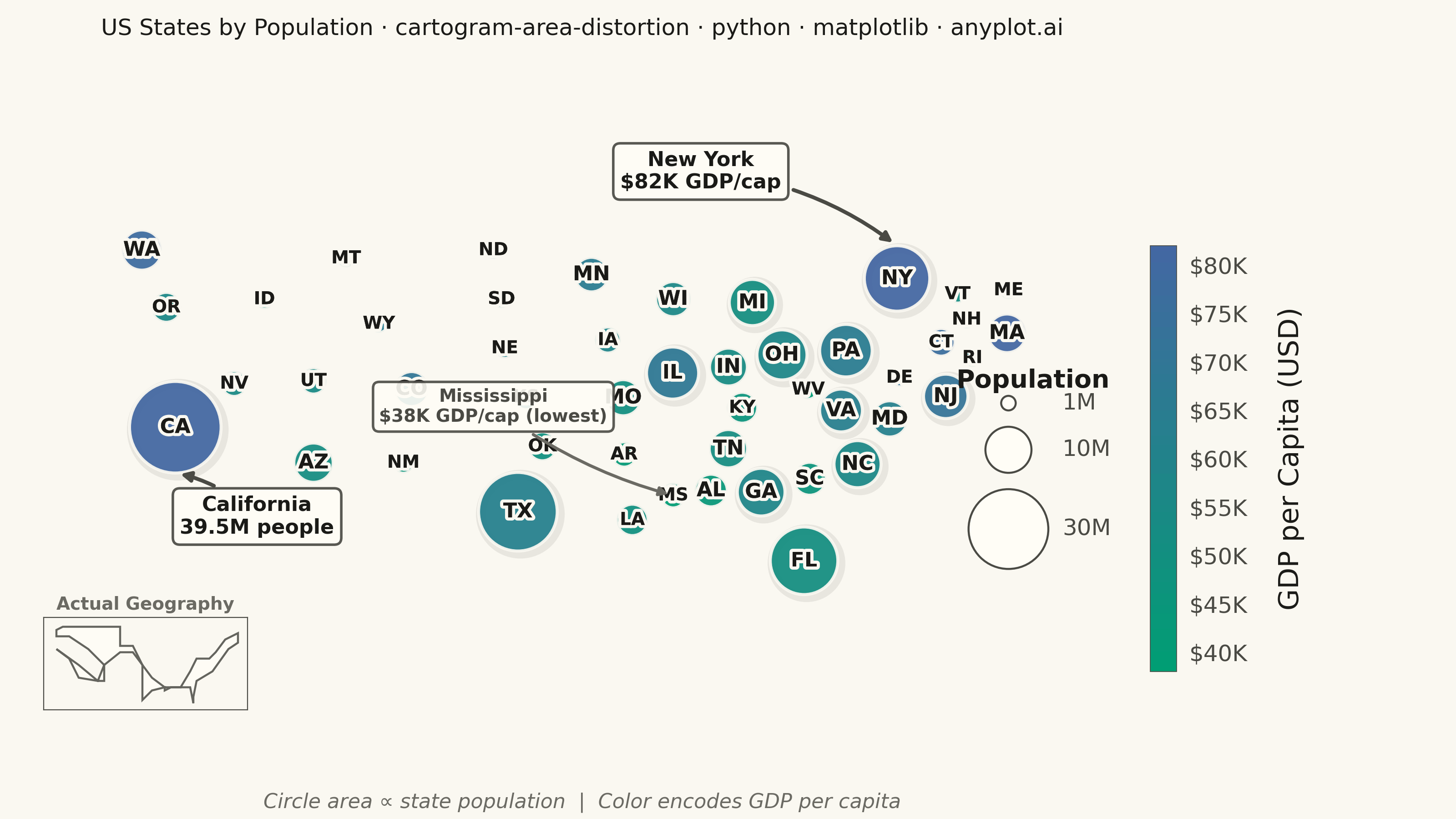
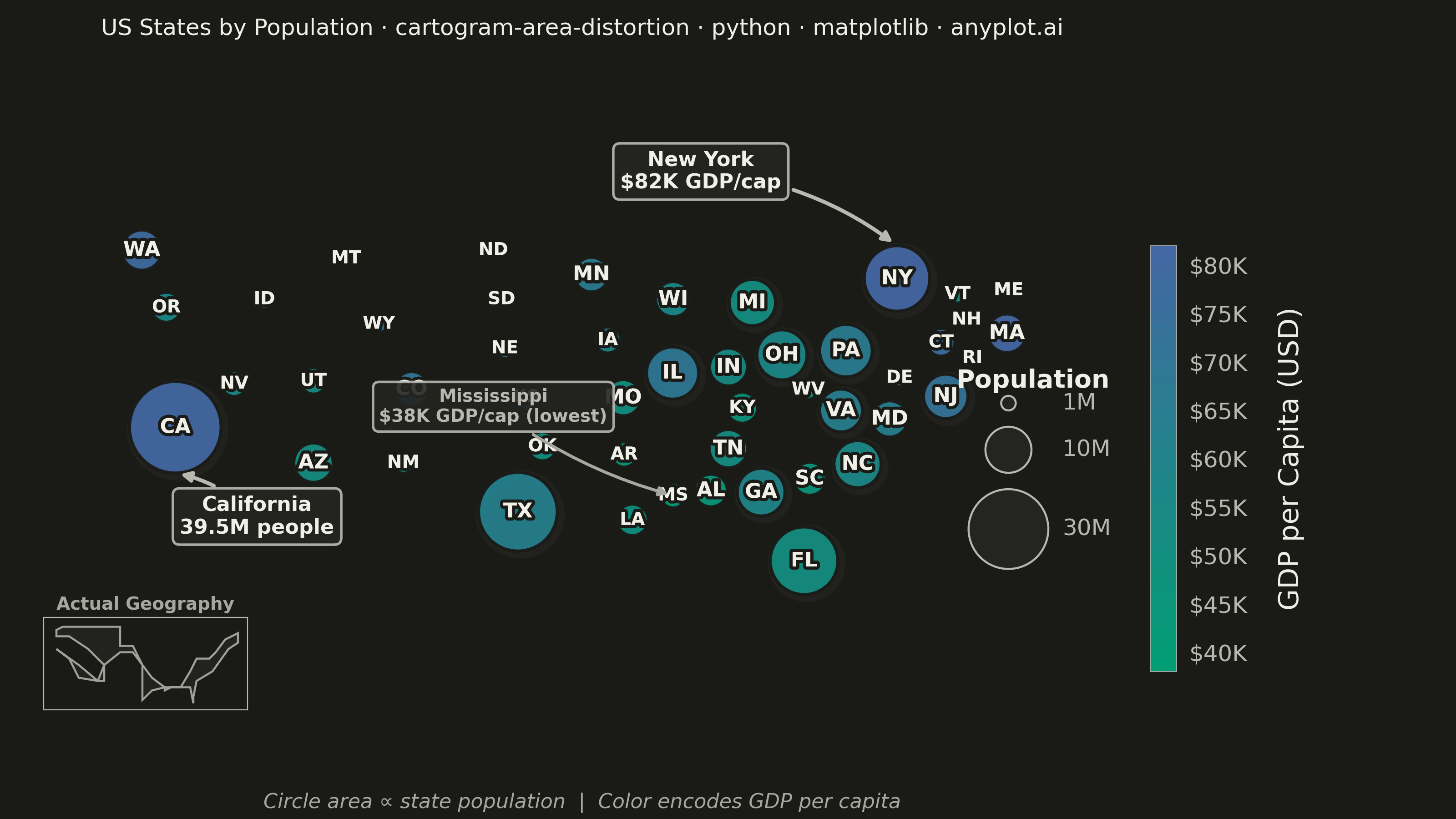
A cartogram distorts geographic regions so that their area becomes proportional to a data variable (e.g., population, GDP, election votes) rather than physical land area. This solves the classic problem of large but sparsely populated areas dominating standard maps, making it easier to compare values across regions at a glance. Contiguous cartograms preserve adjacency and rough shape of regions while rescaling them, famously used in election coverage worldwide.
""" anyplot.ai
cartogram-area-distortion: Cartogram with Area Distortion by Data Value
Library: matplotlib 3.10.9 | Python 3.13.13
Quality: 91/100 | Updated: 2026-06-08
"""

import os

import matplotlib.patches as mpatches
import matplotlib.patheffects as pe
import matplotlib.pyplot as plt
import numpy as np
from matplotlib.cm import ScalarMappable
from matplotlib.collections import PatchCollection
from matplotlib.colors import LinearSegmentedColormap, Normalize


# Theme tokens
THEME = os.getenv("ANYPLOT_THEME", "light")
PAGE_BG = "#FAF8F1" if THEME == "light" else "#1A1A17"
ELEVATED_BG = "#FFFDF6" if THEME == "light" else "#242420"
INK = "#1A1A17" if THEME == "light" else "#F0EFE8"
INK_SOFT = "#4A4A44" if THEME == "light" else "#B8B7B0"
INK_MUTED = "#6B6A63" if THEME == "light" else "#A8A79F"

# Imprint sequential colormap for GDP per capita (single-polarity continuous data)
imprint_seq = LinearSegmentedColormap.from_list("imprint_seq", ["#009E73", "#4467A3"])

# Data — US states with approximate centroids, population (thousands), and GDP per capita
np.random.seed(42)

states = {
    "WA": (-122.0, 47.5, 7615, 78000),
    "OR": (-120.5, 44.0, 4218, 56000),
    "CA": (-119.5, 37.0, 39538, 81000),
    "NV": (-116.8, 39.0, 3104, 55000),
    "ID": (-114.5, 44.5, 1839, 45000),
    "MT": (-109.5, 47.0, 1084, 42000),
    "WY": (-107.5, 43.0, 577, 65000),
    "UT": (-111.5, 39.5, 3272, 54000),
    "CO": (-105.5, 39.0, 5773, 70000),
    "AZ": (-111.5, 34.5, 7279, 52000),
    "NM": (-106.0, 34.5, 2117, 46000),
    "ND": (-100.5, 47.5, 779, 63000),
    "SD": (-100.0, 44.5, 887, 58000),
    "NE": (-99.8, 41.5, 1962, 61000),
    "KS": (-98.5, 38.5, 2937, 55000),
    "OK": (-97.5, 35.5, 3959, 48000),
    "TX": (-99.0, 31.5, 29145, 62000),
    "MN": (-94.5, 46.0, 5640, 65000),
    "IA": (-93.5, 42.0, 3190, 59000),
    "MO": (-92.5, 38.5, 6154, 50000),
    "AR": (-92.5, 35.0, 3012, 41000),
    "LA": (-92.0, 31.0, 4657, 49000),
    "WI": (-89.5, 44.5, 5822, 56000),
    "IL": (-89.0, 40.0, 12812, 68000),
    "MI": (-84.5, 44.0, 10077, 51000),
    "IN": (-86.0, 40.0, 6733, 53000),
    "OH": (-82.5, 40.5, 11799, 57000),
    "KY": (-85.5, 37.8, 4506, 46000),
    "TN": (-86.0, 35.8, 6911, 52000),
    "MS": (-89.5, 32.5, 2961, 38000),
    "AL": (-86.8, 32.8, 5024, 44000),
    "GA": (-83.5, 33.0, 10712, 58000),
    "FL": (-81.5, 28.5, 21538, 51000),
    "SC": (-81.0, 34.0, 5119, 46000),
    "NC": (-79.5, 35.5, 10439, 56000),
    "VA": (-79.0, 37.5, 8631, 63000),
    "WV": (-80.5, 38.8, 1794, 40000),
    "PA": (-77.5, 41.0, 13002, 65000),
    "NY": (-74.5, 43.0, 20201, 82000),
    "NJ": (-74.5, 40.0, 9289, 72000),
    "MD": (-76.5, 39.0, 6177, 62000),
    "DE": (-75.5, 39.0, 990, 73000),
    "CT": (-72.7, 41.6, 3606, 76000),
    "RI": (-71.5, 41.7, 1098, 58000),
    "MA": (-71.8, 42.3, 7029, 82000),
    "VT": (-72.6, 44.0, 643, 52000),
    "NH": (-71.5, 43.5, 1377, 60000),
    "ME": (-69.0, 45.0, 1362, 46000),
}

names = list(states.keys())
lons = np.array([states[s][0] for s in names])
lats = np.array([states[s][1] for s in names])
populations = np.array([states[s][2] for s in names])
gdp_per_capita = np.array([states[s][3] for s in names])

# Scale circle radii proportional to sqrt(population) for area proportionality
max_pop = populations.max()
radii = np.sqrt(populations / max_pop) * 2.8
min_radius = 0.55
radii = np.maximum(radii, min_radius)

# Collision avoidance — more iterations and stronger push for dense NE corridor
adjusted_lons = lons.copy()
adjusted_lats = lats.copy()
ne_states = {"NY", "NJ", "CT", "RI", "MA", "VT", "NH", "ME", "PA", "DE", "MD"}
for _ in range(150):
    for i in range(len(names)):
        for j in range(i + 1, len(names)):
            dx = adjusted_lons[j] - adjusted_lons[i]
            dy = adjusted_lats[j] - adjusted_lats[i]
            dist = np.sqrt(dx**2 + dy**2)
            both_ne = names[i] in ne_states and names[j] in ne_states
            spacing = 1.5 if both_ne else 1.25
            min_dist = (radii[i] + radii[j]) * spacing
            if dist < min_dist and dist > 0:
                overlap = min_dist - dist
                push = overlap / 2
                nx, ny = dx / dist, dy / dist
                strength = 0.55 if both_ne else 0.35
                adjusted_lons[i] -= nx * push * strength
                adjusted_lats[i] -= ny * push * strength
                adjusted_lons[j] += nx * push * strength
                adjusted_lats[j] += ny * push * strength

# Plot
fig = plt.figure(figsize=(8, 4.5), dpi=400, facecolor=PAGE_BG)
ax = fig.add_axes([0.03, 0.08, 0.73, 0.83])
ax.set_facecolor(PAGE_BG)
norm = Normalize(vmin=gdp_per_capita.min(), vmax=gdp_per_capita.max())

# Build circles as PatchCollection for efficient rendering (distinctive matplotlib feature)
shadow_patches = []
main_patches = []
face_colors = []
sort_idx = np.argsort(-populations)

for i in sort_idx:
    color = imprint_seq(norm(gdp_per_capita[i]))
    if populations[i] > 8000:
        shadow = mpatches.Circle((adjusted_lons[i] + 0.15, adjusted_lats[i] - 0.15), radii[i])
        shadow_patches.append(shadow)
    circle = mpatches.Circle((adjusted_lons[i], adjusted_lats[i]), radii[i])
    main_patches.append(circle)
    face_colors.append(color)

if shadow_patches:
    shadow_edgecolor = "#00000012" if THEME == "light" else "#FFFFFF08"
    shadow_col = PatchCollection(
        shadow_patches, facecolors="none", edgecolors=shadow_edgecolor, linewidths=4, zorder=1.8
    )
    ax.add_collection(shadow_col)

main_col = PatchCollection(
    main_patches, facecolors=face_colors, edgecolors=PAGE_BG, linewidths=1.2, alpha=0.94, zorder=2
)
ax.add_collection(main_col)

# State labels — lower threshold to include all notable states including tiny WY/VT
for i in sort_idx:
    if populations[i] > 560:
        fontsize = 8 if populations[i] > 5000 else 7
        ax.text(
            adjusted_lons[i],
            adjusted_lats[i],
            names[i],
            ha="center",
            va="center",
            fontsize=fontsize,
            fontweight="bold",
            color=INK,
            zorder=4,
            path_effects=[pe.withStroke(linewidth=2.5, foreground=PAGE_BG), pe.Normal()],
        )

# Annotations with theme-adaptive styling
ca_idx = names.index("CA")
ax.annotate(
    "California\n39.5M people",
    fontsize=8,
    xy=(adjusted_lons[ca_idx], adjusted_lats[ca_idx] - radii[ca_idx]),
    xytext=(adjusted_lons[ca_idx] + 5, adjusted_lats[ca_idx] - 6.5),
    arrowprops={"arrowstyle": "-|>", "color": INK_SOFT, "lw": 1.5, "connectionstyle": "arc3,rad=0.15"},
    fontweight="bold",
    color=INK,
    ha="center",
    zorder=5,
    bbox={"boxstyle": "round,pad=0.35", "facecolor": ELEVATED_BG, "edgecolor": INK_SOFT, "alpha": 0.92},
)

ny_idx = names.index("NY")
ax.annotate(
    "New York\n$82K GDP/cap",
    fontsize=8,
    xy=(adjusted_lons[ny_idx], adjusted_lats[ny_idx] + radii[ny_idx]),
    xytext=(adjusted_lons[ny_idx] - 12, adjusted_lats[ny_idx] + 5.5),
    arrowprops={"arrowstyle": "-|>", "color": INK_SOFT, "lw": 1.5, "connectionstyle": "arc3,rad=-0.15"},
    fontweight="bold",
    color=INK,
    ha="center",
    zorder=5,
    bbox={"boxstyle": "round,pad=0.35", "facecolor": ELEVATED_BG, "edgecolor": INK_SOFT, "alpha": 0.92},
)

ms_idx = names.index("MS")
ax.annotate(
    "Mississippi\n$38K GDP/cap (lowest)",
    fontsize=7,
    xy=(adjusted_lons[ms_idx], adjusted_lats[ms_idx]),
    xytext=(adjusted_lons[ms_idx] - 11, adjusted_lats[ms_idx] + 4.5),
    arrowprops={"arrowstyle": "-|>", "color": INK_MUTED, "lw": 1.2, "connectionstyle": "arc3,rad=0.1"},
    fontweight="bold",
    color=INK_SOFT,
    ha="center",
    zorder=5,
    bbox={"boxstyle": "round,pad=0.35", "facecolor": ELEVATED_BG, "edgecolor": INK_SOFT, "alpha": 0.9},
)

# Colorbar with theme-adaptive styling
sm = ScalarMappable(cmap=imprint_seq, norm=norm)
sm.set_array([])
cbar_ax = fig.add_axes([0.79, 0.18, 0.018, 0.52])
cbar = fig.colorbar(sm, cax=cbar_ax)
cbar.set_label("GDP per Capita (USD)", fontsize=11, labelpad=12, color=INK)
cbar.ax.tick_params(labelsize=9, length=0, pad=5, labelcolor=INK_SOFT)
cbar.ax.yaxis.set_major_formatter(plt.FuncFormatter(lambda x, _: f"${x / 1000:.0f}K"))
cbar.outline.set_linewidth(0.3)
cbar.outline.set_edgecolor(INK_SOFT)

# Size legend
legend_x = -67.5
legend_y_base = 28.0
ax.text(
    legend_x, legend_y_base + 11.5, "Population", fontsize=10, fontweight="bold", ha="center", va="center", color=INK
)
legend_pops = [30000, 10000, 1000]
legend_labels = ["30M", "10M", "1M"]
legend_radii = [np.sqrt(p / max_pop) * 2.8 for p in legend_pops]

y_pos = legend_y_base
for r, label in zip(legend_radii, legend_labels, strict=True):
    circle_y = y_pos + r
    legend_circle = mpatches.Circle(
        (legend_x - 1.5, circle_y), r, facecolor=ELEVATED_BG, edgecolor=INK_SOFT, linewidth=0.8, zorder=2
    )
    ax.add_patch(legend_circle)
    ax.text(legend_x + 1.8, circle_y, label, fontsize=9, va="center", ha="left", color=INK_SOFT)
    y_pos += r * 2 + 1.0

# Reference map inset (bottom-left corner for geographic comparison)
inset_ax = fig.add_axes([0.03, 0.08, 0.14, 0.22])
us_lon = np.array(
    [
        -124,
        -117,
        -111,
        -109,
        -109,
        -114,
        -120,
        -124,
        -124,
        -122,
        -117,
        -104,
        -104,
        -100,
        -97,
        -94,
        -90,
        -89,
        -82,
        -81,
        -81,
        -80,
        -75,
        -70,
        -67,
        -67,
        -71,
        -74,
        -76,
        -80,
        -82,
        -85,
        -88,
        -90,
        -90,
        -94,
        -97,
        -97,
        -100,
        -104,
        -109,
        -111,
        -117,
        -120,
        -124,
    ]
)
us_lat = np.array(
    [
        42,
        37,
        32,
        32,
        37,
        42,
        46,
        46,
        48,
        49,
        49,
        49,
        43,
        43,
        37,
        33,
        30,
        30,
        30,
        25,
        27,
        32,
        35,
        42,
        44,
        47,
        45,
        41,
        39,
        39,
        35,
        30,
        30,
        29,
        30,
        29,
        26,
        37,
        41,
        41,
        37,
        32,
        33,
        39,
        42,
    ]
)
inset_ax.fill(us_lon, us_lat, color=ELEVATED_BG, edgecolor=INK_SOFT, linewidth=0.8, alpha=0.85)
inset_ax.set_xlim(-128, -64)
inset_ax.set_ylim(23, 52)
inset_ax.set_aspect("equal")
inset_ax.set_title("Actual Geography", fontsize=7, fontweight="bold", color=INK_MUTED, pad=3)
for spine in inset_ax.spines.values():
    spine.set_edgecolor(INK_SOFT)
    spine.set_linewidth(0.4)
inset_ax.set_xticks([])
inset_ax.set_yticks([])
inset_ax.patch.set_facecolor(PAGE_BG)

# Main axes styling
ax.set_xlim(-128, -63)
ax.set_ylim(24, 51)
ax.set_aspect("equal")
for spine in ax.spines.values():
    spine.set_visible(False)
ax.set_xticks([])
ax.set_yticks([])

# Title — full format: {Descriptive} · {spec-id} · {language} · {library} · anyplot.ai
title = "US States by Population · cartogram-area-distortion · python · matplotlib · anyplot.ai"
n = len(title)
title_fontsize = max(8, round(12 * 67 / n)) if n > 67 else 12
fig.text(0.40, 0.965, title, fontsize=title_fontsize, fontweight="medium", ha="center", va="center", color=INK)

# Caption
fig.text(
    0.40,
    0.02,
    "Circle area ∝ state population  |  Color encodes GDP per capita",
    fontsize=8,
    ha="center",
    va="center",
    color=INK_MUTED,
    style="italic",
)

# Save
plt.savefig(f"plot-{THEME}.png", dpi=400, facecolor=PAGE_BG)
Runnable source as JSON, for any HTTP client: https://api.anyplot.ai/specs/cartogram-area-distortion/matplotlib/code. Any spec id and library id listed in llms-full.txt fit the same URL shape; every URL below is complete and callable.
{
  "spec_id": "cartogram-area-distortion",
  "language": "python",
  "library": "matplotlib",
  "page": "https://anyplot.ai/cartogram-area-distortion/python/matplotlib",
  "hub": "https://anyplot.ai/cartogram-area-distortion",
  "code_json": "https://api.anyplot.ai/specs/cartogram-area-distortion/matplotlib/code",
  "spec_json": "https://api.anyplot.ai/specs/cartogram-area-distortion",
  "render_light_png": "https://storage.googleapis.com/anyplot-images/plots/cartogram-area-distortion/python/matplotlib/plot-light.png",
  "render_dark_png": "https://storage.googleapis.com/anyplot-images/plots/cartogram-area-distortion/python/matplotlib/plot-dark.png",
  "quality_score": 91.0,
  "license": "MIT",
  "guide": "https://anyplot.ai/llms.txt"
}
Part of Cartogram with Area Distortion by Data Value on anyplot.ai.