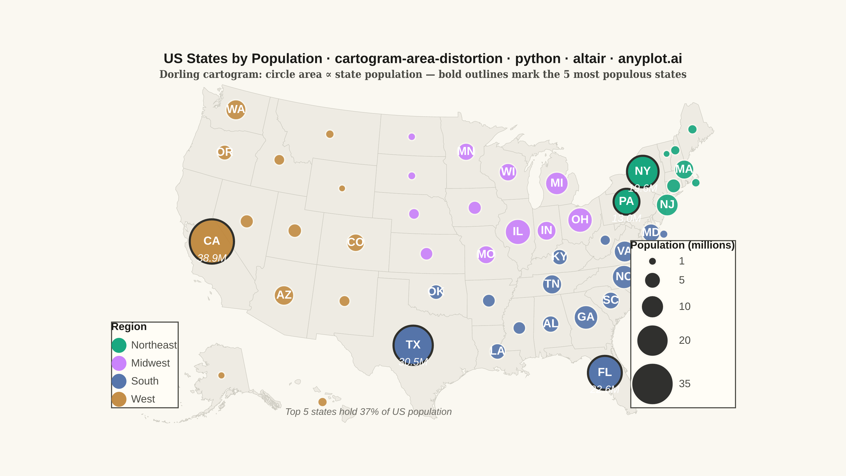
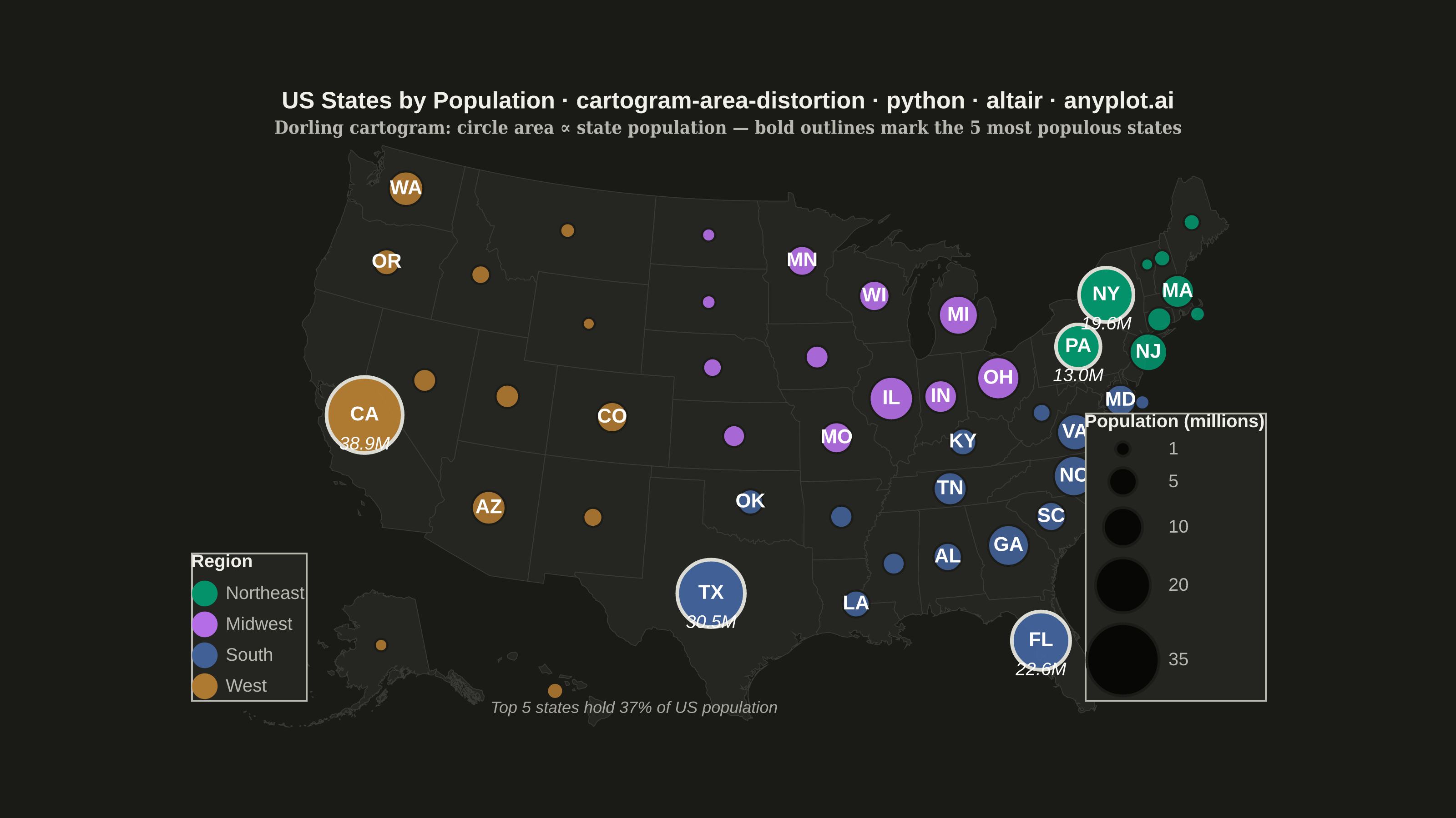
A cartogram distorts geographic regions so that their area becomes proportional to a data variable (e.g., population, GDP, election votes) rather than physical land area. This solves the classic problem of large but sparsely populated areas dominating standard maps, making it easier to compare values across regions at a glance. Contiguous cartograms preserve adjacency and rough shape of regions while rescaling them, famously used in election coverage worldwide.
""" anyplot.ai
cartogram-area-distortion: Cartogram with Area Distortion by Data Value
Library: altair 6.2.1 | Python 3.13.13
Quality: 85/100 | Updated: 2026-06-08
"""

import os
import sys


# Remove '' and this file's directory from sys.path so 'import altair' resolves
# to the installed package, not this file (which shares the library's name)
_here = os.path.dirname(os.path.abspath(__file__))
sys.path = [p for p in sys.path if p not in ("", _here)]

import altair as alt
import pandas as pd
from PIL import Image


# Theme tokens (Imprint palette — see prompts/default-style-guide.md)
THEME = os.getenv("ANYPLOT_THEME", "light")
PAGE_BG = "#FAF8F1" if THEME == "light" else "#1A1A17"
ELEVATED_BG = "#FFFDF6" if THEME == "light" else "#242420"
INK = "#1A1A17" if THEME == "light" else "#F0EFE8"
INK_SOFT = "#4A4A44" if THEME == "light" else "#B8B7B0"
INK_MUTED = "#6B6A63" if THEME == "light" else "#A8A79F"
REF_FILL = "#EEEBE3" if THEME == "light" else "#252521"
REF_STROKE = "#CCCAC0" if THEME == "light" else "#3A3A36"

# Imprint palette — positions 1-4 for four US Census regions
IMPRINT_PALETTE = ["#009E73", "#C475FD", "#4467A3", "#BD8233", "#AE3030", "#2ABCCD", "#954477", "#99B314"]
region_order = ["Northeast", "Midwest", "South", "West"]
region_colors = IMPRINT_PALETTE[:4]

# Data - US states (2023 population estimates, millions) and geographic centroids
states = pd.DataFrame(
    [
        {"state": "AL", "name": "Alabama", "pop": 5.1, "lat": 32.8, "lon": -86.8, "region": "South"},
        {"state": "AK", "name": "Alaska", "pop": 0.7, "lat": 64.2, "lon": -153.5, "region": "West"},
        {"state": "AZ", "name": "Arizona", "pop": 7.4, "lat": 34.3, "lon": -111.7, "region": "West"},
        {"state": "AR", "name": "Arkansas", "pop": 3.0, "lat": 34.9, "lon": -92.4, "region": "South"},
        {"state": "CA", "name": "California", "pop": 38.9, "lat": 37.2, "lon": -119.5, "region": "West"},
        {"state": "CO", "name": "Colorado", "pop": 5.9, "lat": 39.0, "lon": -105.5, "region": "West"},
        {"state": "CT", "name": "Connecticut", "pop": 3.6, "lat": 41.6, "lon": -72.7, "region": "Northeast"},
        {"state": "DE", "name": "Delaware", "pop": 1.0, "lat": 38.2, "lon": -74.8, "region": "South"},
        {"state": "FL", "name": "Florida", "pop": 22.6, "lat": 28.6, "lon": -82.5, "region": "South"},
        {"state": "GA", "name": "Georgia", "pop": 11.0, "lat": 33.0, "lon": -83.5, "region": "South"},
        {"state": "HI", "name": "Hawaii", "pop": 1.4, "lat": 20.5, "lon": -157.5, "region": "West"},
        {"state": "ID", "name": "Idaho", "pop": 2.0, "lat": 44.4, "lon": -114.6, "region": "West"},
        {"state": "IL", "name": "Illinois", "pop": 12.5, "lat": 40.0, "lon": -89.2, "region": "Midwest"},
        {"state": "IN", "name": "Indiana", "pop": 6.9, "lat": 39.9, "lon": -86.3, "region": "Midwest"},
        {"state": "IA", "name": "Iowa", "pop": 3.2, "lat": 42.0, "lon": -93.5, "region": "Midwest"},
        {"state": "KS", "name": "Kansas", "pop": 2.9, "lat": 38.5, "lon": -98.4, "region": "Midwest"},
        {"state": "KY", "name": "Kentucky", "pop": 4.5, "lat": 37.8, "lon": -85.3, "region": "South"},
        {"state": "LA", "name": "Louisiana", "pop": 4.6, "lat": 31.0, "lon": -91.8, "region": "South"},
        {"state": "ME", "name": "Maine", "pop": 1.4, "lat": 45.4, "lon": -69.2, "region": "Northeast"},
        {"state": "MD", "name": "Maryland", "pop": 6.2, "lat": 38.5, "lon": -76.0, "region": "South"},
        {"state": "MA", "name": "Massachusetts", "pop": 7.0, "lat": 42.6, "lon": -71.2, "region": "Northeast"},
        {"state": "MI", "name": "Michigan", "pop": 10.0, "lat": 43.4, "lon": -84.7, "region": "Midwest"},
        {"state": "MN", "name": "Minnesota", "pop": 5.7, "lat": 46.3, "lon": -94.3, "region": "Midwest"},
        {"state": "MS", "name": "Mississippi", "pop": 2.9, "lat": 32.7, "lon": -89.7, "region": "South"},
        {"state": "MO", "name": "Missouri", "pop": 6.2, "lat": 38.4, "lon": -92.5, "region": "Midwest"},
        {"state": "MT", "name": "Montana", "pop": 1.1, "lat": 47.0, "lon": -109.6, "region": "West"},
        {"state": "NE", "name": "Nebraska", "pop": 2.0, "lat": 41.5, "lon": -99.8, "region": "Midwest"},
        {"state": "NV", "name": "Nevada", "pop": 3.2, "lat": 39.3, "lon": -116.6, "region": "West"},
        {"state": "NH", "name": "New Hampshire", "pop": 1.4, "lat": 44.2, "lon": -71.6, "region": "Northeast"},
        {"state": "NJ", "name": "New Jersey", "pop": 9.3, "lat": 40.3, "lon": -73.8, "region": "Northeast"},
        {"state": "NM", "name": "New Mexico", "pop": 2.1, "lat": 34.5, "lon": -106.0, "region": "West"},
        {"state": "NY", "name": "New York", "pop": 19.6, "lat": 43.2, "lon": -75.5, "region": "Northeast"},
        {"state": "NC", "name": "N. Carolina", "pop": 10.7, "lat": 35.6, "lon": -79.4, "region": "South"},
        {"state": "ND", "name": "N. Dakota", "pop": 0.8, "lat": 47.4, "lon": -100.4, "region": "Midwest"},
        {"state": "OH", "name": "Ohio", "pop": 11.8, "lat": 40.4, "lon": -82.8, "region": "Midwest"},
        {"state": "OK", "name": "Oklahoma", "pop": 4.0, "lat": 35.6, "lon": -97.4, "region": "South"},
        {"state": "OR", "name": "Oregon", "pop": 4.2, "lat": 44.0, "lon": -120.5, "region": "West"},
        {"state": "PA", "name": "Pennsylvania", "pop": 13.0, "lat": 41.2, "lon": -77.8, "region": "Northeast"},
        {"state": "RI", "name": "Rhode Island", "pop": 1.1, "lat": 41.4, "lon": -70.4, "region": "Northeast"},
        {"state": "SC", "name": "S. Carolina", "pop": 5.4, "lat": 34.0, "lon": -81.0, "region": "South"},
        {"state": "SD", "name": "S. Dakota", "pop": 0.9, "lat": 44.4, "lon": -100.2, "region": "Midwest"},
        {"state": "TN", "name": "Tennessee", "pop": 7.1, "lat": 35.8, "lon": -86.3, "region": "South"},
        {"state": "TX", "name": "Texas", "pop": 30.5, "lat": 31.5, "lon": -99.4, "region": "South"},
        {"state": "UT", "name": "Utah", "pop": 3.4, "lat": 39.3, "lon": -111.7, "region": "West"},
        {"state": "VT", "name": "Vermont", "pop": 0.6, "lat": 44.1, "lon": -72.6, "region": "Northeast"},
        {"state": "VA", "name": "Virginia", "pop": 8.6, "lat": 37.5, "lon": -78.9, "region": "South"},
        {"state": "WA", "name": "Washington", "pop": 7.8, "lat": 47.4, "lon": -120.5, "region": "West"},
        {"state": "WV", "name": "W. Virginia", "pop": 1.8, "lat": 38.6, "lon": -80.6, "region": "South"},
        {"state": "WI", "name": "Wisconsin", "pop": 5.9, "lat": 44.6, "lon": -89.8, "region": "Midwest"},
        {"state": "WY", "name": "Wyoming", "pop": 0.6, "lat": 43.0, "lon": -107.5, "region": "West"},
    ]
)

states = states.sort_values("pop", ascending=False).reset_index(drop=True)
states["rank"] = states.index + 1
states["pop_label"] = states["pop"].apply(lambda x: f"{x:.1f}M")
top5 = states.head(5)
labeled_states = states[states["pop"] >= 4.0].copy()

# Reference map - faint state outlines for geographic context
us_topo_url = "https://cdn.jsdelivr.net/npm/vega-datasets@2/data/us-10m.json"
us_states_topo = alt.topo_feature(us_topo_url, "states")

background = (
    alt.Chart(us_states_topo).mark_geoshape(fill=REF_FILL, stroke=REF_STROKE, strokeWidth=0.4).project(type="albersUsa")
)

# Dorling cartogram — single layer with alt.condition to highlight top-5 states
top5_names = ["California", "Texas", "Florida", "New York", "Pennsylvania"]
is_top5 = alt.FieldOneOfPredicate(field="name", oneOf=top5_names)

circles = (
    alt.Chart(states)
    .mark_circle()
    .encode(
        longitude="lon:Q",
        latitude="lat:Q",
        size=alt.Size(
            "pop:Q",
            scale=alt.Scale(domain=[0.5, 40], range=[40, 1800]),
            legend=alt.Legend(
                title="Population (millions)",
                titleFontSize=10,
                labelFontSize=10,
                orient="bottom-right",
                offset=15,
                values=[1, 5, 10, 20, 35],
            ),
        ),
        color=alt.Color(
            "region:N",
            scale=alt.Scale(domain=region_order, range=region_colors),
            legend=alt.Legend(
                title="Region",
                titleFontSize=10,
                labelFontSize=10,
                symbolSize=200,
                symbolStrokeWidth=0,
                orient="bottom-left",
                offset=15,
            ),
        ),
        opacity=alt.condition(is_top5, alt.value(0.90), alt.value(0.82)),
        stroke=alt.condition(is_top5, alt.value(INK), alt.value(PAGE_BG)),
        strokeWidth=alt.condition(is_top5, alt.value(2.0), alt.value(1.2)),
        tooltip=[
            alt.Tooltip("name:N", title="State"),
            alt.Tooltip("pop:Q", title="Population (M)", format=".1f"),
            alt.Tooltip("region:N", title="Region"),
        ],
    )
    .project(type="albersUsa")
)

# State abbreviation labels for states >= 4M population
labels = (
    alt.Chart(labeled_states)
    .mark_text(fontSize=11, fontWeight="bold", color="#FFFFFF")
    .encode(longitude="lon:Q", latitude="lat:Q", text="state:N")
    .project(type="albersUsa")
)

# Population values below labels for top 5 states
pop_labels = (
    alt.Chart(top5)
    .mark_text(fontSize=10, color="#FFFFFF", dy=16, fontStyle="italic")
    .encode(longitude="lon:Q", latitude="lat:Q", text="pop_label:N")
    .project(type="albersUsa")
)

# Annotation — key insight placed in lower map area
annotation_data = pd.DataFrame([{"text": "Top 5 states hold 37% of US population", "lat": 25.5, "lon": -110.0}])
annotation = (
    alt.Chart(annotation_data)
    .mark_text(fontSize=9, fontStyle="italic", color=INK_MUTED, align="left")
    .encode(longitude="lon:Q", latitude="lat:Q", text="text:N")
    .project(type="albersUsa")
)

# Title with scaled font size for the longer mandated title string
title_str = "US States by Population · cartogram-area-distortion · python · altair · anyplot.ai"
n = len(title_str)
ratio = 67 / n if n > 67 else 1.0
title_fontsize = max(11, round(16 * ratio))

# Combine all layers
chart = (
    (background + circles + labels + pop_labels + annotation)
    .properties(
        width=620,
        height=320,
        title=alt.Title(
            text=title_str,
            subtitle="Dorling cartogram: circle area ∝ state population — bold outlines mark the 5 most populous states",
            fontSize=title_fontsize,
            subtitleFontSize=10,
            subtitleColor=INK_SOFT,
            anchor="middle",
        ),
    )
    .configure_view(strokeWidth=0, fill=PAGE_BG)
    .configure(background=PAGE_BG)
    .configure_legend(fillColor=ELEVATED_BG, strokeColor=INK_SOFT, labelColor=INK_SOFT, titleColor=INK)
    .configure_title(color=INK)
)

# Save PNG
chart.save(f"plot-{THEME}.png", scale_factor=4.0)

# Pad to exact 3200×1800 target (vl-convert inner-view padding leaves canvas short)
TW, TH = 3200, 1800
_img = Image.open(f"plot-{THEME}.png").convert("RGB")
_w, _h = _img.size
if _w > TW or _h > TH:
    raise SystemExit(
        f"altair vl-convert produced {_w}×{_h}, exceeds target {TW}×{TH}. "
        "Shrink chart width/height values and re-render."
    )
if _w < TW or _h < TH:
    _canvas = Image.new("RGB", (TW, TH), PAGE_BG)
    _canvas.paste(_img, ((TW - _w) // 2, (TH - _h) // 2))
    _canvas.save(f"plot-{THEME}.png")

# Save interactive HTML
chart.save(f"plot-{THEME}.html")
Runnable source as JSON, for any HTTP client: https://api.anyplot.ai/specs/cartogram-area-distortion/altair/code. Any spec id and library id listed in llms-full.txt fit the same URL shape; every URL below is complete and callable.
{
  "spec_id": "cartogram-area-distortion",
  "language": "python",
  "library": "altair",
  "page": "https://anyplot.ai/cartogram-area-distortion/python/altair",
  "hub": "https://anyplot.ai/cartogram-area-distortion",
  "code_json": "https://api.anyplot.ai/specs/cartogram-area-distortion/altair/code",
  "spec_json": "https://api.anyplot.ai/specs/cartogram-area-distortion",
  "render_light_png": "https://storage.googleapis.com/anyplot-images/plots/cartogram-area-distortion/python/altair/plot-light.png",
  "render_dark_png": "https://storage.googleapis.com/anyplot-images/plots/cartogram-area-distortion/python/altair/plot-dark.png",
  "interactive_light_html": "https://storage.googleapis.com/anyplot-images/plots/cartogram-area-distortion/python/altair/plot-light.html",
  "interactive_dark_html": "https://storage.googleapis.com/anyplot-images/plots/cartogram-area-distortion/python/altair/plot-dark.html",
  "quality_score": 85.0,
  "license": "MIT",
  "guide": "https://anyplot.ai/llms.txt"
}
Part of Cartogram with Area Distortion by Data Value on anyplot.ai.