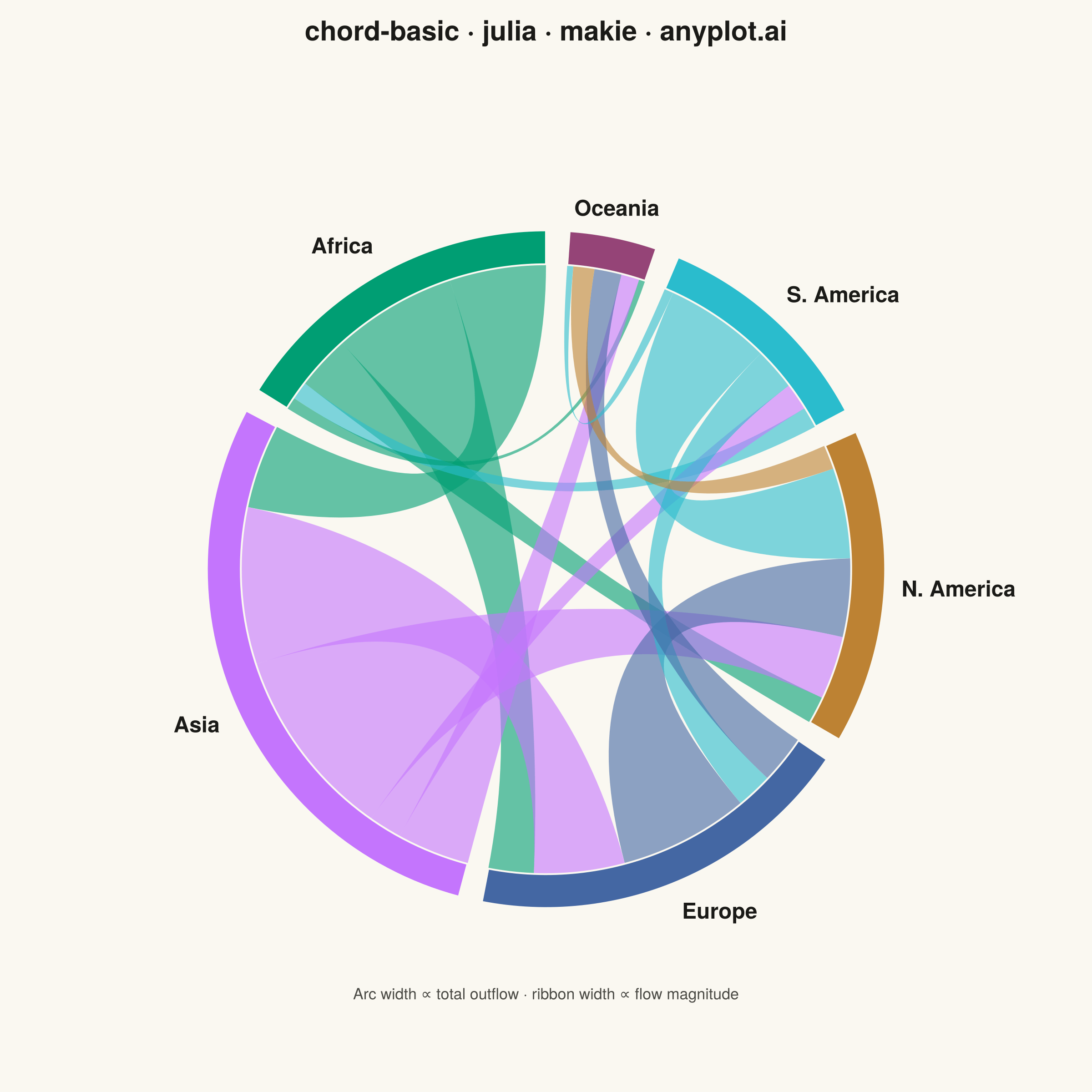
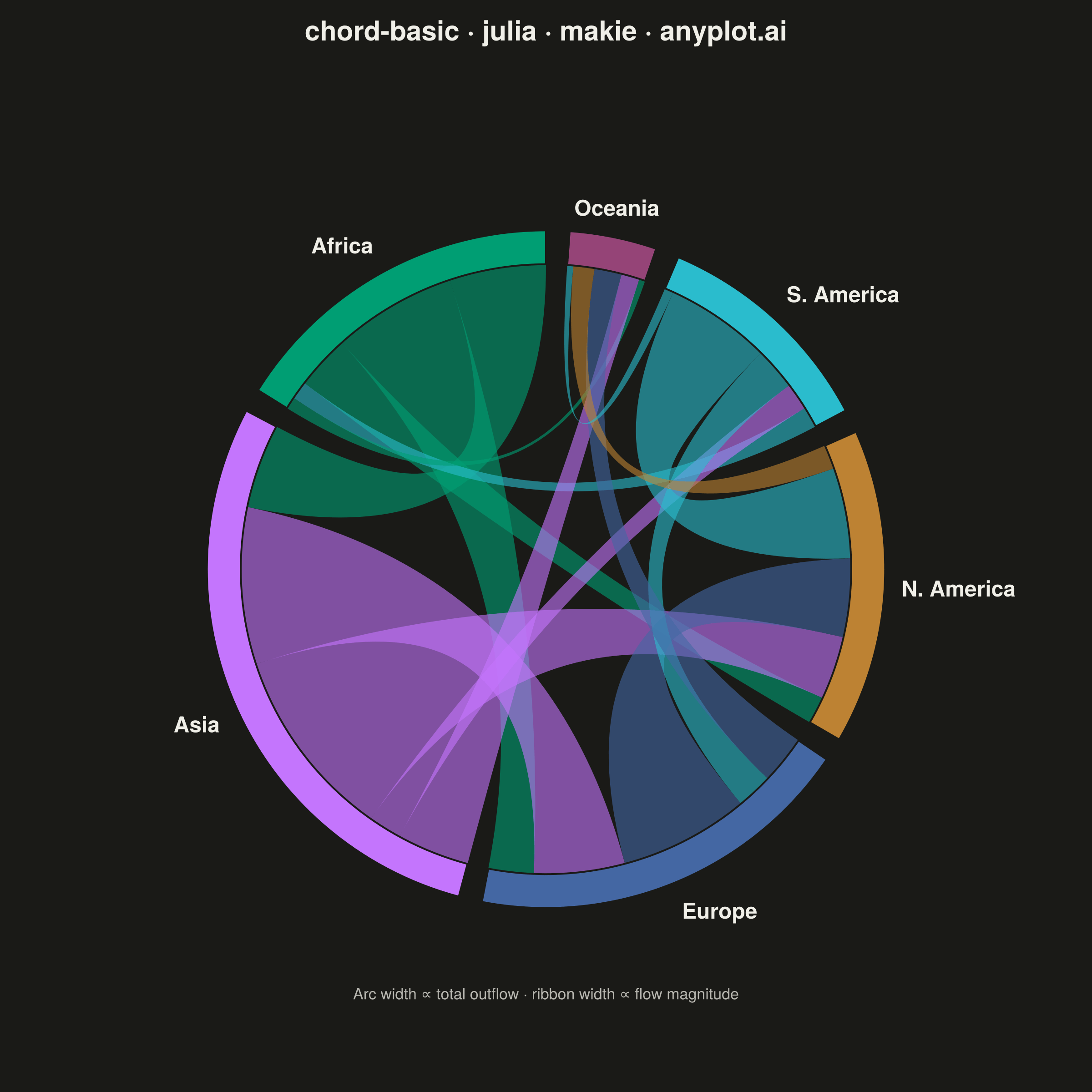
A chord diagram displays relationships or flows between entities arranged around a circle's perimeter. Arcs (chords) connect related entities, with chord width proportional to the flow magnitude. This visualization excels at revealing the overall structure of connections and identifying the strongest relationships within a system.
# anyplot.ai
# chord-basic: Basic Chord Diagram
# Library: makie 0.22.10 | Julia 1.11.9
# Quality: 90/100 | Created: 2026-06-17

using CairoMakie
using Colors

# --- Theme tokens (see prompts/default-style-guide.md "Theme-adaptive Chrome") ---
const THEME    = get(ENV, "ANYPLOT_THEME", "light")
const PAGE_BG  = THEME == "light" ? colorant"#FAF8F1" : colorant"#1A1A17"
const INK      = THEME == "light" ? colorant"#1A1A17" : colorant"#F0EFE8"
const INK_SOFT = THEME == "light" ? colorant"#4A4A44" : colorant"#B8B7B0"

# Imprint palette — one distinct hue per region; first series is brand green.
const IMPRINT_PALETTE = [
    colorant"#009E73",  # 1 — brand green
    colorant"#C475FD",  # 2 — lavender
    colorant"#4467A3",  # 3 — blue
    colorant"#BD8233",  # 4 — ochre
    colorant"#2ABCCD",  # 6 — cyan
    colorant"#954477",  # 7 — rose
]

# --- Data: annual migration flows between 6 world regions (thousands of people) ---
regions = ["Africa", "Asia", "Europe", "N. America", "S. America", "Oceania"]

# flow[i, j] = migrants moving from region i to region j (diagonal is unused)
flow = Float64[
    0  320  410  180   60   40    # from Africa
  280    0  520  640  110  240    # from Asia
  150  300    0  430  120  160    # from Europe
   90  210  260    0  300   80    # from N. America
   70   90  140  350    0   30    # from S. America
   20   60   90   70   20    0    # from Oceania
]

# --- Geometry: one arc per region, sized by total throughput (outflow + inflow) ---
# Each arc reserves a separate foot for every directed flow, so i→j and j→i render
# as two distinct, source-tinted chords rather than a single merged ribbon.
n          = length(regions)
gap        = deg2rad(4.0)                          # angular gap between adjacent arcs
throughput = vec(sum(flow, dims = 2)) .+ vec(sum(flow, dims = 1))  # row + column totals
span       = (2π - n * gap) .* throughput ./ sum(throughput)

# Each arc starts at the top (π/2) offset by the spans and gaps that precede it.
arc_start = [π / 2 + sum(span[1:i-1]) + (i - 1) * gap for i in 1:n]
arc_stop  = arc_start .+ span

# Walk each arc once, laying down an outgoing foot then an incoming foot per partner.
out_foot = fill((0.0, 0.0), n, n)   # out_foot[i, j] = sub-arc on i carrying flow i→j
in_foot  = fill((0.0, 0.0), n, n)   # in_foot[i, j]  = sub-arc on i receiving flow j→i
for i in 1:n
    a = arc_start[i]
    for j in 1:n
        w_out = flow[i, j] / throughput[i] * span[i]
        out_foot[i, j] = (a, a + w_out)
        a += w_out
        w_in = flow[j, i] / throughput[i] * span[i]
        in_foot[i, j] = (a, a + w_in)
        a += w_in
    end
end

# Radii: colored ring sits between r_in and r_out; ribbons attach at r_in.
r_in  = 0.90
r_out = 1.00

# Helpers: a point on a circle, and a quadratic Bézier bowed through the centre.
on_ring = (t, rad) -> Point2f(rad * cos(t), rad * sin(t))
bezier  = (p0, p2) -> [Point2f((1 - t)^2 * p0[1] + t^2 * p2[1],
                               (1 - t)^2 * p0[2] + t^2 * p2[2]) for t in range(0, 1; length = 48)]

# --- Plot ---
fig = Figure(size = (1200, 1200), backgroundcolor = PAGE_BG)

ax = Axis(
    fig[1, 1];
    title           = "chord-basic · julia · makie · anyplot.ai",
    titlesize       = 30,
    titlecolor      = INK,
    titlegap        = 16,
    backgroundcolor = PAGE_BG,
    aspect          = DataAspect(),
)
hidespines!(ax)
hidedecorations!(ax)
limits!(ax, -1.5, 1.5, -1.5, 1.5)

# One ribbon per directed flow, tinted by its source. Largest flows are drawn
# first so the thin tail flows stay readable on top, keeping the core legible.
order = sort([(i, j) for i in 1:n, j in 1:n if flow[i, j] > 0];
    by = ij -> flow[ij[1], ij[2]], rev = true)
for (i, j) in order
    a0, a1 = out_foot[i, j]                  # source foot on region i
    b0, b1 = in_foot[j, i]                   # target foot on region j
    foot_i = [on_ring(t, r_in) for t in range(a0, a1; length = 12)]
    foot_j = [on_ring(t, r_in) for t in range(b0, b1; length = 12)]
    ribbon = vcat(
        foot_i,
        bezier(foot_i[end], foot_j[1]),
        foot_j,
        bezier(foot_j[end], foot_i[1]),
    )
    poly!(ax, ribbon; color = (IMPRINT_PALETTE[i], 0.5), strokewidth = 0)
end

# Colored arc segment per region (outer ring forward, inner ring back).
for i in 1:n
    ang   = range(arc_start[i], arc_stop[i]; length = 64)
    outer = [on_ring(t, r_out) for t in ang]
    inner = [on_ring(t, r_in) for t in reverse(ang)]
    poly!(ax, vcat(outer, inner);
        color = IMPRINT_PALETTE[i], strokecolor = PAGE_BG, strokewidth = 2)
end

# Region labels, placed just outside the ring and anchored by quadrant.
for i in 1:n
    mid = (arc_start[i] + arc_stop[i]) / 2
    cx, cy = cos(mid), sin(mid)
    ha = abs(cx) < 0.35 ? :center : (cx > 0 ? :left : :right)
    va = abs(cy) < 0.35 ? :center : (cy > 0 ? :bottom : :top)
    text!(ax, 1.05 * cx, 1.05 * cy;
        text = regions[i], align = (ha, va), color = INK,
        fontsize = 24, font = :bold)
end

# Footnote: clarify the encoding without faking interactivity.
text!(ax, 0.0, -1.28;
    text = "Arc width ∝ total flow · each ribbon is one direction, tinted by its source region",
    align = (:center, :bottom), color = INK_SOFT, fontsize = 17)

# --- Save ---
save("plot-$(THEME).png", fig; px_per_unit = 2)
Runnable source as JSON, for any HTTP client: https://api.anyplot.ai/specs/chord-basic/makie/code. Any spec id and library id listed in llms-full.txt fit the same URL shape; every URL below is complete and callable.
{
  "spec_id": "chord-basic",
  "language": "julia",
  "library": "makie",
  "page": "https://anyplot.ai/chord-basic/julia/makie",
  "hub": "https://anyplot.ai/chord-basic",
  "code_json": "https://api.anyplot.ai/specs/chord-basic/makie/code",
  "spec_json": "https://api.anyplot.ai/specs/chord-basic",
  "render_light_png": "https://storage.googleapis.com/anyplot-images/plots/chord-basic/julia/makie/plot-light.png",
  "render_dark_png": "https://storage.googleapis.com/anyplot-images/plots/chord-basic/julia/makie/plot-dark.png",
  "quality_score": 90.0,
  "license": "MIT",
  "guide": "https://anyplot.ai/llms.txt"
}
Part of Basic Chord Diagram on anyplot.ai.