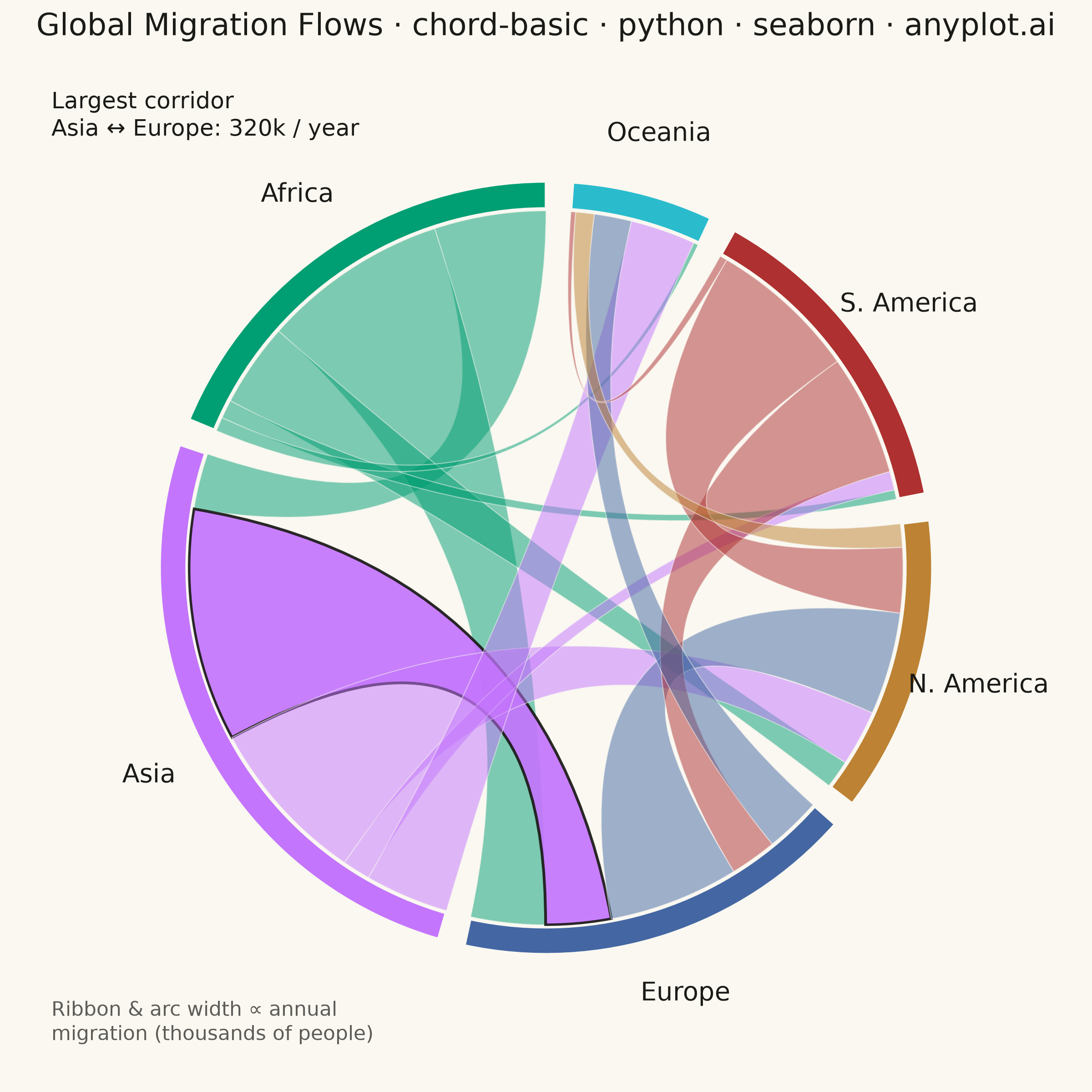
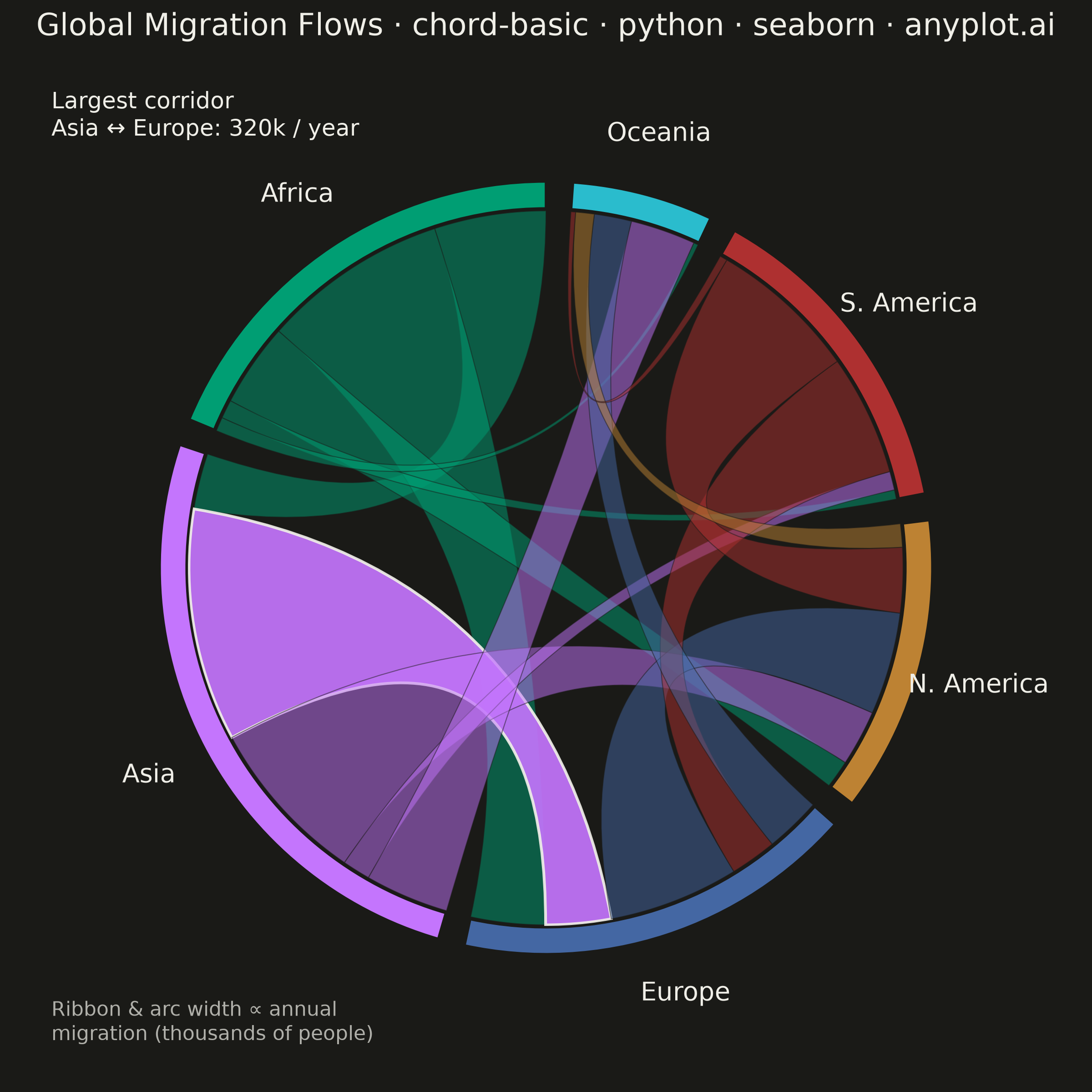
A chord diagram displays relationships or flows between entities arranged around a circle's perimeter. Arcs (chords) connect related entities, with chord width proportional to the flow magnitude. This visualization excels at revealing the overall structure of connections and identifying the strongest relationships within a system.
""" anyplot.ai
chord-basic: Basic Chord Diagram
Library: seaborn 0.13.2 | Python 3.13.13
Quality: 85/100 | Created: 2026-06-17
"""

import os

import matplotlib.pyplot as plt
import numpy as np
import seaborn as sns
from matplotlib.patches import PathPatch, Wedge
from matplotlib.path import Path


# Theme tokens (see prompts/default-style-guide.md "Theme-adaptive Chrome")
THEME = os.getenv("ANYPLOT_THEME", "light")
PAGE_BG = "#FAF8F1" if THEME == "light" else "#1A1A17"
INK = "#1A1A17" if THEME == "light" else "#F0EFE8"

# Imprint palette — one distinct hue per continent, first entity always #009E73
IMPRINT_PALETTE = ["#009E73", "#C475FD", "#4467A3", "#BD8233", "#AE3030", "#2ABCCD"]

sns.set_theme(style="white", rc={"figure.facecolor": PAGE_BG, "axes.facecolor": PAGE_BG, "text.color": INK})
sns.set_palette(IMPRINT_PALETTE)

# Data — directed migration flows between 6 continents (thousands of people / year)
continents = ["Africa", "Asia", "Europe", "N. America", "S. America", "Oceania"]
flows = np.array(
    [
        [0, 120, 200, 90, 20, 15],  # from Africa
        [60, 0, 250, 180, 30, 90],  # from Asia
        [80, 70, 0, 140, 50, 60],  # from Europe
        [30, 60, 110, 0, 70, 25],  # from N. America
        [10, 20, 130, 160, 0, 8],  # from S. America
        [5, 70, 40, 20, 5, 0],  # from Oceania
    ],
    dtype=float,
)

# Geometry — lay each continent on an arc proportional to its total outgoing flow
n = len(continents)
gap = np.deg2rad(4)  # angular gap between continent arcs
group_total = flows.sum(axis=1)
scale = (2 * np.pi - n * gap) / flows.sum()

group_start = np.zeros(n)
cursor = np.pi / 2  # start at the top of the circle
for i in range(n):
    group_start[i] = cursor
    cursor += group_total[i] * scale + gap

# Sub-arc spans: slice (i, j) reserves the angle for the i -> j flow on i's arc
sub_start = np.zeros((n, n))
sub_end = np.zeros((n, n))
for i in range(n):
    a = group_start[i]
    for j in range(n):
        sub_start[i, j] = a
        a += flows[i, j] * scale
        sub_end[i, j] = a

# Focal corridor — the largest bidirectional pair, highlighted to anchor the story
combined = flows + flows.T
focal = np.unravel_index(np.argmax(np.triu(combined, 1)), combined.shape)

# Plot — square canvas: figsize=(6, 6) dpi=400 -> 2400 x 2400 px
fig, ax = plt.subplots(figsize=(6, 6), dpi=400, facecolor=PAGE_BG)
ax.set_facecolor(PAGE_BG)
ax.set_aspect("equal")
ax.axis("off")

outer_r = 1.0
ring_w = 0.07
ribbon_r = outer_r - ring_w - 0.006
arc_res = 24  # points used to trace each circular arc segment

# Ribbons — one chord per continent pair, width at each end = that direction's flow
for i in range(n):
    for j in range(i + 1, n):
        if flows[i, j] == 0 and flows[j, i] == 0:
            continue

        # colour the chord by the dominant migration direction's source
        src = i if flows[i, j] >= flows[j, i] else j

        a0, a1 = sub_start[i, j], sub_end[i, j]
        b0, b1 = sub_start[j, i], sub_end[j, i]

        verts = []
        codes = []

        # arc along i's slice: a0 -> a1
        ts = np.linspace(a0, a1, arc_res)
        arc_i = ribbon_r * np.column_stack([np.cos(ts), np.sin(ts)])
        verts.append(arc_i[0])
        codes.append(Path.MOVETO)
        for p in arc_i[1:]:
            verts.append(p)
            codes.append(Path.LINETO)

        # quadratic Bezier through the centre: a1 -> b0
        verts.append((0.0, 0.0))
        codes.append(Path.CURVE3)
        verts.append((ribbon_r * np.cos(b0), ribbon_r * np.sin(b0)))
        codes.append(Path.CURVE3)

        # arc along j's slice: b0 -> b1
        ts = np.linspace(b0, b1, arc_res)
        arc_j = ribbon_r * np.column_stack([np.cos(ts), np.sin(ts)])
        for p in arc_j[1:]:
            verts.append(p)
            codes.append(Path.LINETO)

        # quadratic Bezier through the centre: b1 -> a0 (closes the ribbon)
        verts.append((0.0, 0.0))
        codes.append(Path.CURVE3)
        verts.append((ribbon_r * np.cos(a0), ribbon_r * np.sin(a0)))
        codes.append(Path.CURVE3)
        verts.append((0.0, 0.0))
        codes.append(Path.CLOSEPOLY)

        # emphasise the focal corridor; let the rest recede so the story reads
        is_focal = {i, j} == {focal[0], focal[1]}
        ax.add_patch(
            PathPatch(
                Path(verts, codes),
                facecolor=IMPRINT_PALETTE[src],
                edgecolor=INK if is_focal else PAGE_BG,
                linewidth=1.1 if is_focal else 0.4,
                alpha=0.92 if is_focal else 0.5,
            )
        )

# Outer ring — one solid arc per continent for identity, plus a label
for i in range(n):
    theta1 = np.rad2deg(group_start[i])
    theta2 = np.rad2deg(group_start[i] + group_total[i] * scale)
    ax.add_patch(
        Wedge(
            (0, 0),
            outer_r,
            theta1,
            theta2,
            width=ring_w,
            facecolor=IMPRINT_PALETTE[i],
            edgecolor=PAGE_BG,
            linewidth=1.0,
        )
    )

    mid = np.deg2rad((theta1 + theta2) / 2)
    ax.text(
        1.16 * np.cos(mid),
        1.16 * np.sin(mid),
        continents[i],
        ha="center",
        va="center",
        fontsize=10,
        fontweight="medium",
        color=INK,
    )

# Corner annotations — the inscribed circle leaves the canvas corners empty, so
# use them for the focal insight (top-left) and the flow-magnitude scale (bottom-left)
fa, fb = continents[focal[0]], continents[focal[1]]
ax.text(
    -1.28,
    1.24,
    f"Largest corridor\n{fa} ↔ {fb}: {int(combined[focal])}k / year",
    ha="left",
    va="top",
    fontsize=9,
    fontweight="medium",
    color=INK,
)
ax.text(
    -1.28,
    -1.24,
    "Ribbon & arc width ∝ annual\nmigration (thousands of people)",
    ha="left",
    va="bottom",
    fontsize=8,
    color=INK,
    alpha=0.7,
)

ax.set_xlim(-1.3, 1.3)
ax.set_ylim(-1.3, 1.3)

# Title — scale fontsize off the 67-char baseline so the long title never overflows
title = "Global Migration Flows · chord-basic · python · seaborn · anyplot.ai"
title_fs = max(8, round(12 * 67 / len(title))) if len(title) > 67 else 12
ax.set_title(title, fontsize=title_fs, fontweight="medium", color=INK, pad=12)

# Save — bbox_inches stays default (None) so figsize x dpi gives exactly 2400x2400
fig.subplots_adjust(left=0.02, right=0.98, top=0.94, bottom=0.02)
plt.savefig(f"plot-{THEME}.png", dpi=400, facecolor=PAGE_BG)
Runnable source as JSON, for any HTTP client: https://api.anyplot.ai/specs/chord-basic/seaborn/code. Any spec id and library id listed in llms-full.txt fit the same URL shape; every URL below is complete and callable.
{
  "spec_id": "chord-basic",
  "language": "python",
  "library": "seaborn",
  "page": "https://anyplot.ai/chord-basic/python/seaborn",
  "hub": "https://anyplot.ai/chord-basic",
  "code_json": "https://api.anyplot.ai/specs/chord-basic/seaborn/code",
  "spec_json": "https://api.anyplot.ai/specs/chord-basic",
  "render_light_png": "https://storage.googleapis.com/anyplot-images/plots/chord-basic/python/seaborn/plot-light.png",
  "render_dark_png": "https://storage.googleapis.com/anyplot-images/plots/chord-basic/python/seaborn/plot-dark.png",
  "quality_score": 85.0,
  "license": "MIT",
  "guide": "https://anyplot.ai/llms.txt"
}
Part of Basic Chord Diagram on anyplot.ai.