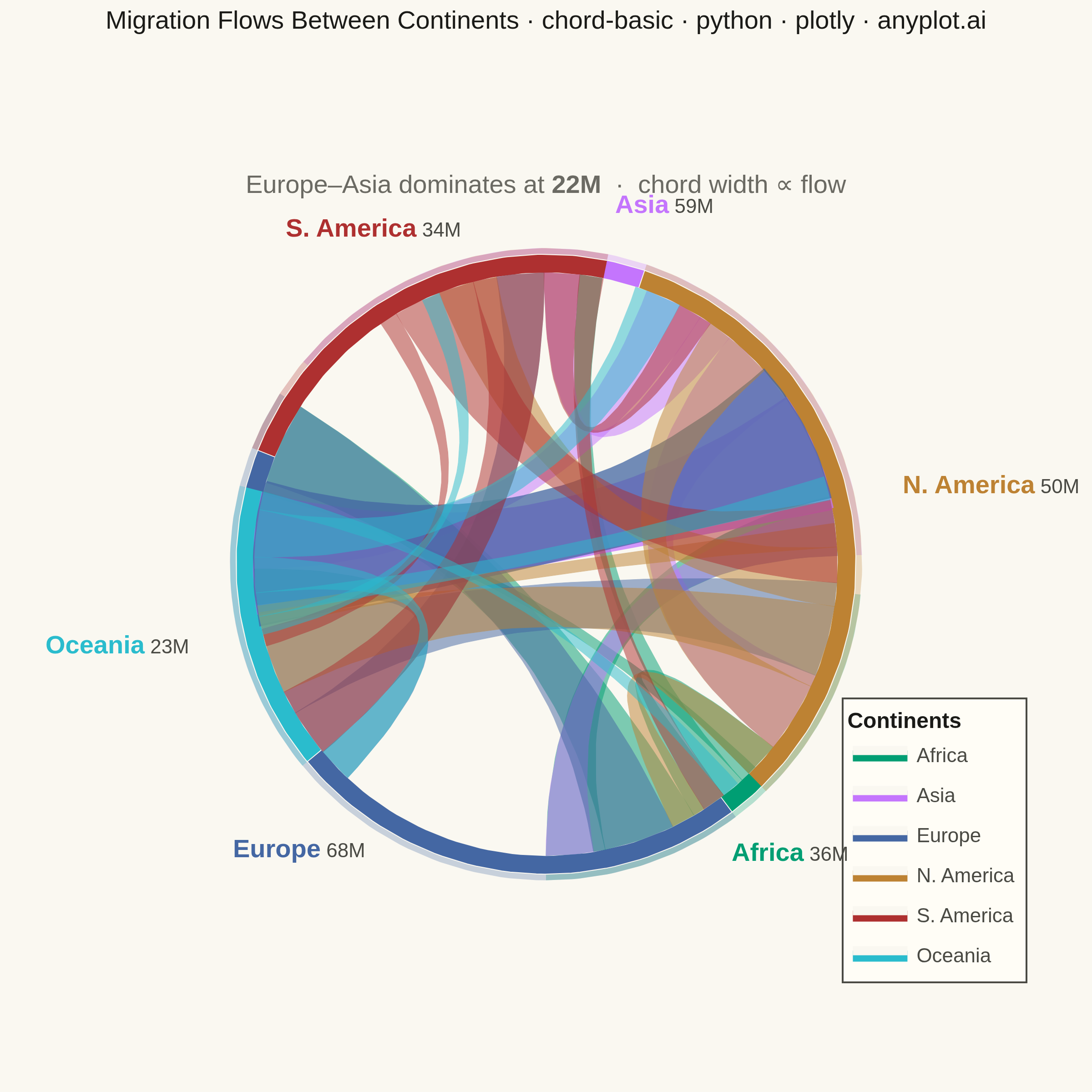
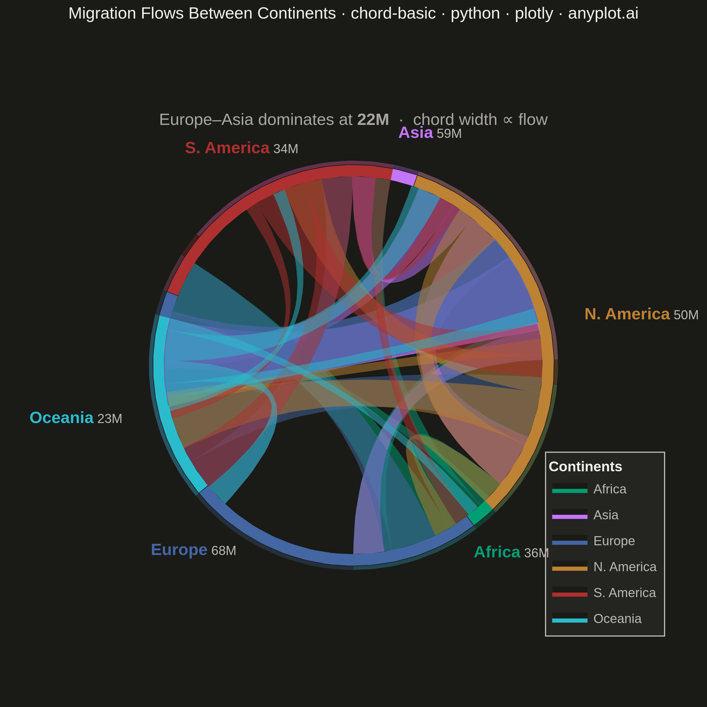
A chord diagram displays relationships or flows between entities arranged around a circle's perimeter. Arcs (chords) connect related entities, with chord width proportional to the flow magnitude. This visualization excels at revealing the overall structure of connections and identifying the strongest relationships within a system.
""" anyplot.ai
chord-basic: Basic Chord Diagram
Library: plotly 6.8.0 | Python 3.13.13
Quality: 89/100 | Updated: 2026-06-17
"""

import os

import numpy as np
import plotly.graph_objects as go


# Theme tokens
THEME = os.getenv("ANYPLOT_THEME", "light")
PAGE_BG = "#FAF8F1" if THEME == "light" else "#1A1A17"
ELEVATED_BG = "#FFFDF6" if THEME == "light" else "#242420"
INK = "#1A1A17" if THEME == "light" else "#F0EFE8"
INK_SOFT = "#4A4A44" if THEME == "light" else "#B8B7B0"
INK_MUTED = "#6B6A63" if THEME == "light" else "#A8A79F"

# Imprint palette — 6 hues for 6 entities (first series always #009E73)
COLORS = ["#009E73", "#C475FD", "#4467A3", "#BD8233", "#AE3030", "#2ABCCD"]
COLORS_DIM = [
    "rgba(0,158,115,0.28)",
    "rgba(196,117,253,0.28)",
    "rgba(68,103,163,0.28)",
    "rgba(189,130,51,0.28)",
    "rgba(174,48,48,0.28)",
    "rgba(42,188,205,0.28)",
]

# Data: Migration flows between 6 continents (bidirectional, millions of people)
continents = ["Africa", "Asia", "Europe", "N. America", "S. America", "Oceania"]
n = len(continents)

flow_matrix = np.array(
    [
        [0, 5, 8, 3, 2, 1],  # Africa to others
        [4, 0, 10, 7, 3, 5],  # Asia to others
        [7, 12, 0, 8, 4, 3],  # Europe to others
        [3, 6, 7, 0, 5, 2],  # N. America to others
        [2, 3, 6, 7, 0, 1],  # S. America to others
        [1, 4, 3, 2, 1, 0],  # Oceania to others
    ]
)

# Totals per continent and dominant corridor for storytelling
totals = flow_matrix.sum(axis=0) + flow_matrix.sum(axis=1)
total_flow = flow_matrix.sum()

max_flow_idx = np.unravel_index(np.argmax(flow_matrix + flow_matrix.T), flow_matrix.shape)
dominant_src, dominant_tgt = max_flow_idx
dominant_flow = flow_matrix[dominant_src, dominant_tgt] + flow_matrix[dominant_tgt, dominant_src]

# Arc positions around the circle
gap = 0.02
arc_starts = []
arc_ends = []
current_pos = 0
for total in totals:
    arc_starts.append(current_pos)
    arc_ends.append(current_pos + (total / total_flow) * (1 - n * gap))
    current_pos = arc_ends[-1] + gap

# Figure
fig = go.Figure()

# Outer translucent ring + inner solid arc for each continent
for i in range(n):
    angles_outer = np.linspace(2 * np.pi * arc_starts[i] - np.pi / 2, 2 * np.pi * arc_ends[i] - np.pi / 2, 100)
    angles_rev = angles_outer[::-1]

    fig.add_trace(
        go.Scatter(
            x=np.concatenate([1.02 * np.cos(angles_outer), 0.98 * np.cos(angles_rev)]),
            y=np.concatenate([1.02 * np.sin(angles_outer), 0.98 * np.sin(angles_rev)]),
            fill="toself",
            fillcolor=COLORS_DIM[i],
            line={"color": "rgba(0,0,0,0)", "width": 0},
            hoverinfo="skip",
            showlegend=False,
        )
    )

    fig.add_trace(
        go.Scatter(
            x=np.concatenate([np.cos(angles_outer), 0.94 * np.cos(angles_rev)]),
            y=np.concatenate([np.sin(angles_outer), 0.94 * np.sin(angles_rev)]),
            fill="toself",
            fillcolor=COLORS[i],
            line={"color": PAGE_BG, "width": 0.5},
            hovertemplate=(
                f"<b>{continents[i]}</b><br>"
                f"Outgoing: {int(flow_matrix[i].sum())}M<br>"
                f"Incoming: {int(flow_matrix[:, i].sum())}M<br>"
                f"Total: {int(totals[i])}M people"
                "<extra></extra>"
            ),
            name=continents[i],
            showlegend=True,
            legendgroup=continents[i],
        )
    )

# Chords — width proportional to flow magnitude
min_chord_width = 0.010
for i in range(n):
    src_pos = arc_starts[i]
    for j in range(n):
        if i == j or flow_matrix[i, j] == 0:
            continue

        flow = flow_matrix[i, j]
        chord_width = max((flow / total_flow) * (1 - n * gap), min_chord_width)

        is_dominant = (i == dominant_src and j == dominant_tgt) or (i == dominant_tgt and j == dominant_src)
        opacity = 0.75 if is_dominant else 0.50
        line_width = 2.0 if is_dominant else 0.3

        tgt_base = arc_starts[j]
        tgt_offset = sum(
            max((flow_matrix[k, j] / total_flow) * (1 - n * gap), min_chord_width)
            for k in range(i)
            if flow_matrix[k, j] > 0
        )

        src_angle1 = 2 * np.pi * src_pos - np.pi / 2
        src_angle2 = 2 * np.pi * (src_pos + chord_width) - np.pi / 2
        sx1, sy1 = 0.94 * np.cos(src_angle1), 0.94 * np.sin(src_angle1)
        sx2, sy2 = 0.94 * np.cos(src_angle2), 0.94 * np.sin(src_angle2)

        tgt_start = tgt_base + tgt_offset
        tgt_end = tgt_start + chord_width
        tgt_angle1 = 2 * np.pi * tgt_start - np.pi / 2
        tgt_angle2 = 2 * np.pi * tgt_end - np.pi / 2
        tx1, ty1 = 0.94 * np.cos(tgt_angle1), 0.94 * np.sin(tgt_angle1)
        tx2, ty2 = 0.94 * np.cos(tgt_angle2), 0.94 * np.sin(tgt_angle2)

        src_angles = np.linspace(src_angle1, src_angle2, 20)
        t = np.linspace(0, 1, 40)
        bez1_x = (1 - t) ** 2 * sx2 + 2 * (1 - t) * t * 0 + t**2 * tx1
        bez1_y = (1 - t) ** 2 * sy2 + 2 * (1 - t) * t * 0 + t**2 * ty1

        tgt_angles = np.linspace(tgt_angle1, tgt_angle2, 20)
        bez2_x = (1 - t) ** 2 * tx2 + 2 * (1 - t) * t * 0 + t**2 * sx1
        bez2_y = (1 - t) ** 2 * ty2 + 2 * (1 - t) * t * 0 + t**2 * sy1

        chord_x = np.concatenate([0.94 * np.cos(src_angles), bez1_x, 0.94 * np.cos(tgt_angles), bez2_x])
        chord_y = np.concatenate([0.94 * np.sin(src_angles), bez1_y, 0.94 * np.sin(tgt_angles), bez2_y])

        fig.add_trace(
            go.Scatter(
                x=chord_x,
                y=chord_y,
                fill="toself",
                fillcolor=COLORS[i],
                opacity=opacity,
                line={"color": COLORS[i], "width": line_width},
                hovertemplate=(
                    f"<b>{continents[i]} → {continents[j]}</b><br>"
                    f"Flow: {flow}M people<br>"
                    f"Share: {flow / total_flow * 100:.1f}% of total"
                    "<extra></extra>"
                ),
                showlegend=False,
                hoveron="fills",
            )
        )

        src_pos += chord_width

# Continent labels at perimeter
for i in range(n):
    mid_pos = (arc_starts[i] + arc_ends[i]) / 2
    angle = 2 * np.pi * mid_pos - np.pi / 2
    lx = 1.17 * np.cos(angle)
    ly = 1.17 * np.sin(angle)
    angle_deg = np.degrees(angle) % 360

    if 45 < angle_deg < 135:
        xanchor, yanchor = "center", "bottom"
    elif 135 <= angle_deg < 225:
        xanchor, yanchor = "right", "middle"
    elif 225 <= angle_deg < 315:
        xanchor, yanchor = "center", "top"
    else:
        xanchor, yanchor = "left", "middle"

    fig.add_annotation(
        x=lx,
        y=ly,
        text=(f"<b>{continents[i]}</b><span style='font-size:11px;color:{INK_SOFT}'> {int(totals[i])}M</span>"),
        font={"size": 14, "color": COLORS[i], "family": "Arial, Helvetica, sans-serif"},
        showarrow=False,
        xanchor=xanchor,
        yanchor=yanchor,
    )

# Subtitle
fig.add_annotation(
    text=f"Europe–Asia dominates at <b>{dominant_flow}M</b>  ·  chord width ∝ flow",
    xref="paper",
    yref="paper",
    x=0.5,
    y=0.965,
    showarrow=False,
    font={"size": 14, "color": INK_MUTED, "family": "Arial, Helvetica, sans-serif"},
    xanchor="center",
)

# Title with scaled fontsize for long string
title = "Migration Flows Between Continents · chord-basic · python · plotly · anyplot.ai"
title_len = len(title)
title_fontsize = round(16 * 67 / title_len) if title_len > 67 else 16
title_fontsize = max(title_fontsize, 11)

fig.update_layout(
    autosize=False,
    title={
        "text": title,
        "font": {"size": title_fontsize, "color": INK, "family": "Arial Black, Arial, sans-serif"},
        "x": 0.5,
        "xanchor": "center",
        "y": 0.99,
        "yanchor": "top",
    },
    xaxis={"showgrid": False, "zeroline": False, "showticklabels": False, "showline": False, "range": [-1.38, 1.38]},
    yaxis={
        "showgrid": False,
        "zeroline": False,
        "showticklabels": False,
        "showline": False,
        "range": [-1.38, 1.38],
        "scaleanchor": "x",
    },
    paper_bgcolor=PAGE_BG,
    plot_bgcolor=PAGE_BG,
    font={"color": INK},
    showlegend=True,
    legend={
        "font": {"size": 11, "family": "Arial, Helvetica, sans-serif", "color": INK_SOFT},
        "title": {"text": "<b>Continents</b>", "font": {"size": 12, "color": INK}},
        "x": 0.99,
        "y": 0.01,
        "xanchor": "right",
        "yanchor": "bottom",
        "bgcolor": ELEVATED_BG,
        "bordercolor": INK_SOFT,
        "borderwidth": 1,
        "tracegroupgap": 3,
        "itemsizing": "constant",
    },
    margin={"l": 30, "r": 30, "t": 75, "b": 55},
    hovermode="closest",
    hoverlabel={
        "bgcolor": ELEVATED_BG,
        "bordercolor": INK_SOFT,
        "font": {"size": 13, "family": "Arial, Helvetica, sans-serif", "color": INK},
    },
)

# Save — square canvas (2400×2400) ideal for circular chord diagram
fig.write_image(f"plot-{THEME}.png", width=600, height=600, scale=4)
fig.write_html(f"plot-{THEME}.html", include_plotlyjs="cdn")
Runnable source as JSON, for any HTTP client: https://api.anyplot.ai/specs/chord-basic/plotly/code. Any spec id and library id listed in llms-full.txt fit the same URL shape; every URL below is complete and callable.
{
  "spec_id": "chord-basic",
  "language": "python",
  "library": "plotly",
  "page": "https://anyplot.ai/chord-basic/python/plotly",
  "hub": "https://anyplot.ai/chord-basic",
  "code_json": "https://api.anyplot.ai/specs/chord-basic/plotly/code",
  "spec_json": "https://api.anyplot.ai/specs/chord-basic",
  "render_light_png": "https://storage.googleapis.com/anyplot-images/plots/chord-basic/python/plotly/plot-light.png",
  "render_dark_png": "https://storage.googleapis.com/anyplot-images/plots/chord-basic/python/plotly/plot-dark.png",
  "interactive_light_html": "https://storage.googleapis.com/anyplot-images/plots/chord-basic/python/plotly/plot-light.html",
  "interactive_dark_html": "https://storage.googleapis.com/anyplot-images/plots/chord-basic/python/plotly/plot-dark.html",
  "quality_score": 89.0,
  "license": "MIT",
  "guide": "https://anyplot.ai/llms.txt"
}
Part of Basic Chord Diagram on anyplot.ai.