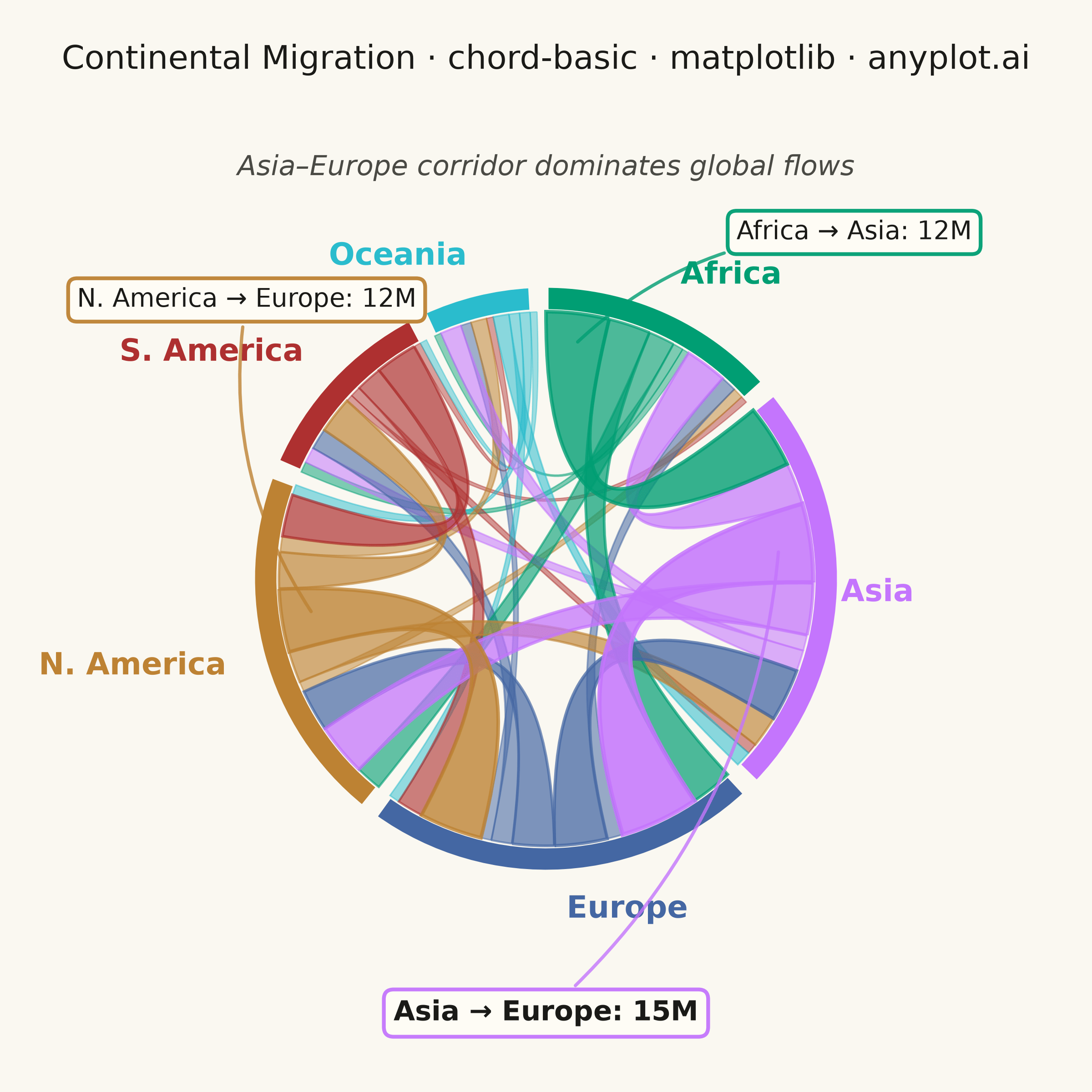
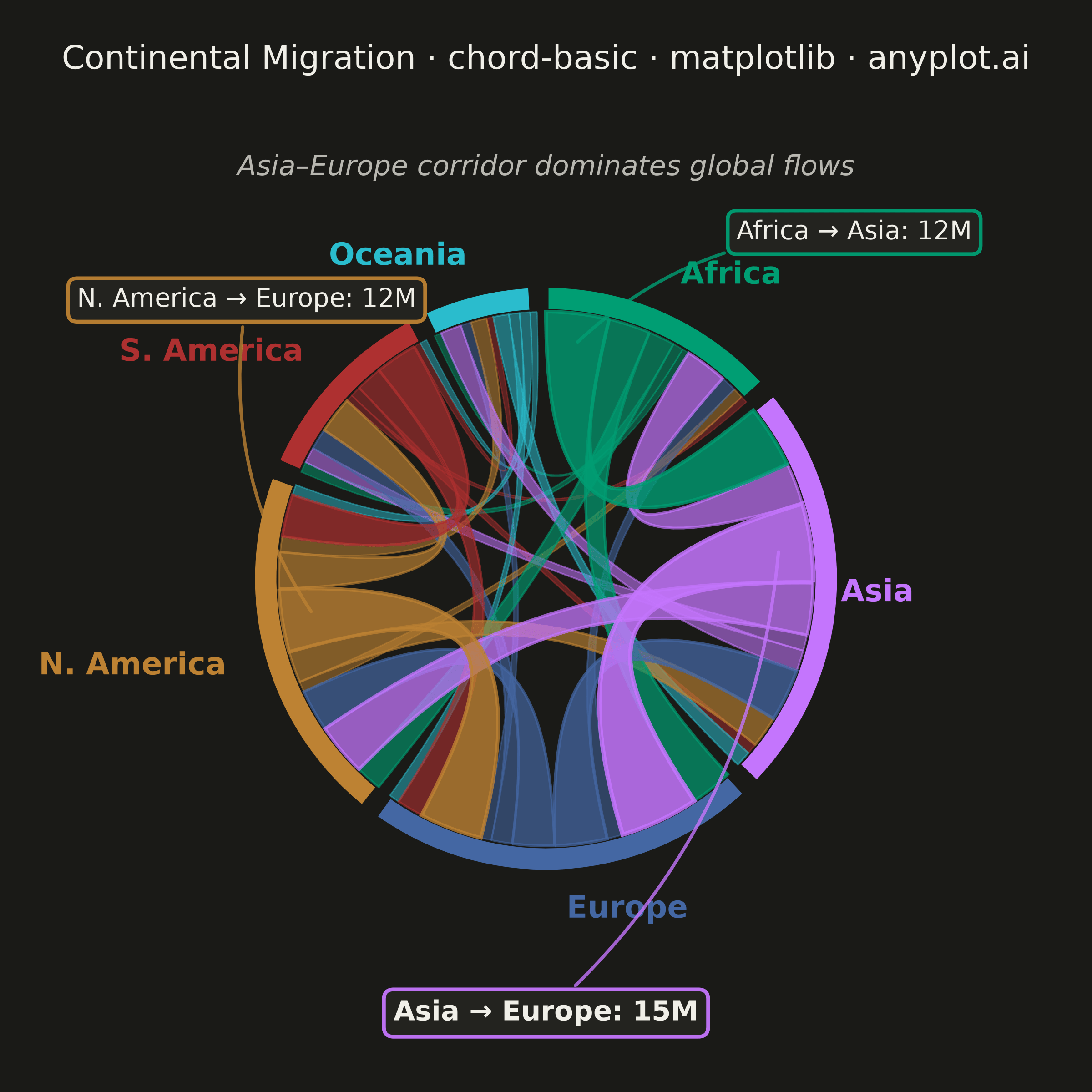
A chord diagram displays relationships or flows between entities arranged around a circle's perimeter. Arcs (chords) connect related entities, with chord width proportional to the flow magnitude. This visualization excels at revealing the overall structure of connections and identifying the strongest relationships within a system.
""" anyplot.ai
chord-basic: Basic Chord Diagram
Library: matplotlib 3.11.0 | Python 3.13.13
Quality: 93/100 | Created: 2026-06-17
"""

import os

import matplotlib.patches as mpatches
import matplotlib.pyplot as plt
import numpy as np
from matplotlib.path import Path


# Theme-adaptive chrome (Imprint palette) — only chrome flips between themes,
# the categorical data colors stay constant.
THEME = os.getenv("ANYPLOT_THEME", "light")
PAGE_BG = "#FAF8F1" if THEME == "light" else "#1A1A17"
ELEVATED_BG = "#FFFDF6" if THEME == "light" else "#242420"
INK = "#1A1A17" if THEME == "light" else "#F0EFE8"
INK_SOFT = "#4A4A44" if THEME == "light" else "#B8B7B0"
INK_MUTED = "#6B6A63" if THEME == "light" else "#A8A79F"

# Imprint categorical palette — first series ALWAYS brand green (#009E73)
IMPRINT_PALETTE = ["#009E73", "#C475FD", "#4467A3", "#BD8233", "#AE3030", "#2ABCCD", "#954477", "#99B314"]

# Data: Migration flows between continents (in millions)
entities = ["Africa", "Asia", "Europe", "N. America", "S. America", "Oceania"]
n = len(entities)

flow_matrix = np.array(
    [
        [0, 12, 8, 5, 2, 1],  # From Africa
        [8, 0, 15, 10, 3, 4],  # From Asia
        [3, 10, 0, 8, 4, 2],  # From Europe
        [2, 6, 12, 0, 7, 3],  # From N. America
        [1, 2, 5, 8, 0, 1],  # From S. America
        [0, 3, 2, 2, 1, 0],  # From Oceania
    ]
)

colors = IMPRINT_PALETTE[:n]

# Calculate entity totals and arc geometry
totals = flow_matrix.sum(axis=1) + flow_matrix.sum(axis=0)
total_flow = totals.sum()
gap_deg = 3
available_deg = 360 - gap_deg * n
arc_spans = (totals / total_flow) * available_deg

# Start angles (clockwise from top)
start_angles = np.zeros(n)
angle = 90
for i in range(n):
    start_angles[i] = angle
    angle -= arc_spans[i] + gap_deg

# Plot — square canvas (2400x2400) for the circular chart
fig, ax = plt.subplots(figsize=(6, 6), dpi=400, subplot_kw={"aspect": "equal"})
fig.set_facecolor(PAGE_BG)
ax.set_xlim(-1.6, 1.6)
ax.set_ylim(-1.6, 1.6)
ax.set_facecolor(PAGE_BG)
ax.axis("off")

radius = 1.0
arc_width = 0.09
inner_r = radius - arc_width

# Draw outer arcs — separators use the page bg so segments read cleanly on both themes
for i in range(n):
    theta1 = start_angles[i] - arc_spans[i]
    theta2 = start_angles[i]
    wedge = mpatches.Wedge(
        (0, 0), radius, theta1, theta2, width=arc_width, facecolor=colors[i], edgecolor=PAGE_BG, linewidth=2
    )
    ax.add_patch(wedge)

    # Label placement — color-coordinated with the entity arc
    mid = np.radians((theta1 + theta2) / 2)
    lx, ly = (radius + 0.13) * np.cos(mid), (radius + 0.13) * np.sin(mid)
    mid_deg = np.degrees(mid) % 360
    ha = (
        "center"
        if mid_deg < 15 or mid_deg > 345 or 165 < mid_deg < 195
        else ("right" if 90 < mid_deg < 270 else "left")
    )
    ax.text(lx, ly, entities[i], fontsize=12, fontweight="bold", ha=ha, va="center", color=colors[i])

# Track angular position within each arc for chord placement
unit_angles = arc_spans / totals

# Pre-compute chord positions to avoid cursor interference from draw order
min_chord_deg = 1.5  # minimum angular span for visibility
chord_params = []
pos_cursors = start_angles.copy()
for i in range(n):
    for j in range(n):
        if i != j and flow_matrix[i, j] > 0:
            flow = flow_matrix[i, j]
            src_span = max(flow * unit_angles[i], min_chord_deg)
            src_end = pos_cursors[i]
            src_start = src_end - src_span
            pos_cursors[i] = src_start

            tgt_span = max(flow * unit_angles[j], min_chord_deg)
            tgt_end = pos_cursors[j]
            tgt_start = tgt_end - tgt_span
            pos_cursors[j] = tgt_start

            chord_params.append(
                {
                    "i": i,
                    "j": j,
                    "src_start": src_start,
                    "src_end": src_end,
                    "tgt_start": tgt_start,
                    "tgt_end": tgt_end,
                    "color": colors[i],
                    "flow": flow,
                }
            )

# Sort by flow magnitude so largest chords render on top
chord_params.sort(key=lambda c: c["flow"])

# Draw chords using cubic Bezier paths
n_arc_pts = 30
ctrl_factor = 0.25
flow_max = flow_matrix.max()

for c in chord_params:
    s1, e1 = np.radians(c["src_start"]), np.radians(c["src_end"])
    s2, e2 = np.radians(c["tgt_start"]), np.radians(c["tgt_end"])

    arc1_t = np.linspace(s1, e1, n_arc_pts)
    arc1 = np.column_stack([inner_r * np.cos(arc1_t), inner_r * np.sin(arc1_t)])

    arc2_t = np.linspace(s2, e2, n_arc_pts)
    arc2 = np.column_stack([inner_r * np.cos(arc2_t), inner_r * np.sin(arc2_t)])

    # Build closed path: arc1 -> bezier -> arc2 -> bezier -> close
    verts = [arc1[0]]
    codes = [Path.MOVETO]

    for pt in arc1[1:]:
        verts.append(pt)
        codes.append(Path.LINETO)

    verts.extend([arc1[-1] * ctrl_factor, arc2[0] * ctrl_factor, arc2[0]])
    codes.extend([Path.CURVE4, Path.CURVE4, Path.CURVE4])

    for pt in arc2[1:]:
        verts.append(pt)
        codes.append(Path.LINETO)

    verts.extend([arc2[-1] * ctrl_factor, arc1[0] * ctrl_factor, arc1[0]])
    codes.extend([Path.CURVE4, Path.CURVE4, Path.CURVE4])

    # Scale alpha and linewidth by flow magnitude for clear visual hierarchy.
    # Floor raised so the smallest flows (e.g. Oceania links) stay legible.
    flow_ratio = c["flow"] / flow_max
    alpha = 0.35 + 0.5 * flow_ratio**0.6
    lw = 0.4 + 1.3 * flow_ratio
    patch = mpatches.PathPatch(
        Path(verts, codes), facecolor=c["color"], edgecolor=c["color"], linewidth=lw, alpha=alpha
    )
    ax.add_patch(patch)

# Annotate the top 3 flows with leader lines connecting each box to its chord
top_flows = sorted(chord_params, key=lambda c: c["flow"], reverse=True)[:3]

# Box anchor positions (outside the ring, in open quadrants)
box_positions = [(0.0, -1.48), (1.05, 1.18), (-1.02, 0.95)]
for rank, c in enumerate(top_flows):
    # Leader-line target: source-ribbon midpoint pulled just inside the arc
    src_mid = np.radians((c["src_start"] + c["src_end"]) / 2)
    tx, ty = inner_r * 0.88 * np.cos(src_mid), inner_r * 0.88 * np.sin(src_mid)

    bx, by = box_positions[rank]
    label = f"{entities[c['i']]} → {entities[c['j']]}: {c['flow']}M"
    fs = 11 if rank == 0 else 10
    ax.annotate(
        label,
        xy=(tx, ty),
        xytext=(bx, by),
        fontsize=fs,
        fontweight="bold" if rank == 0 else "normal",
        ha="center",
        va="center",
        color=INK,
        bbox={
            "boxstyle": "round,pad=0.35",
            "facecolor": ELEVATED_BG,
            "edgecolor": c["color"],
            "alpha": 0.95,
            "linewidth": 1.5,
        },
        arrowprops={
            "arrowstyle": "-",
            "color": c["color"],
            "linewidth": 1.3,
            "alpha": 0.8,
            "connectionstyle": "arc3,rad=0.2",
        },
    )

# Title and subtitle — title fontsize scales with length to avoid overflow
title = "Continental Migration · chord-basic · matplotlib · anyplot.ai"
title_fs = max(8, round(13 * 60 / len(title))) if len(title) > 60 else 13
ax.set_title(title, fontsize=title_fs, fontweight="medium", pad=16, color=INK)
ax.text(
    0,
    1.40,
    "Asia–Europe corridor dominates global flows",
    fontsize=11,
    ha="center",
    va="center",
    color=INK_SOFT,
    fontstyle="italic",
)

fig.subplots_adjust(left=0.04, right=0.96, top=0.90, bottom=0.04)
plt.savefig(f"plot-{THEME}.png", dpi=400, facecolor=PAGE_BG)
Runnable source as JSON, for any HTTP client: https://api.anyplot.ai/specs/chord-basic/matplotlib/code. Any spec id and library id listed in llms-full.txt fit the same URL shape; every URL below is complete and callable.
{
  "spec_id": "chord-basic",
  "language": "python",
  "library": "matplotlib",
  "page": "https://anyplot.ai/chord-basic/python/matplotlib",
  "hub": "https://anyplot.ai/chord-basic",
  "code_json": "https://api.anyplot.ai/specs/chord-basic/matplotlib/code",
  "spec_json": "https://api.anyplot.ai/specs/chord-basic",
  "render_light_png": "https://storage.googleapis.com/anyplot-images/plots/chord-basic/python/matplotlib/plot-light.png",
  "render_dark_png": "https://storage.googleapis.com/anyplot-images/plots/chord-basic/python/matplotlib/plot-dark.png",
  "quality_score": 93.0,
  "license": "MIT",
  "guide": "https://anyplot.ai/llms.txt"
}
Part of Basic Chord Diagram on anyplot.ai.