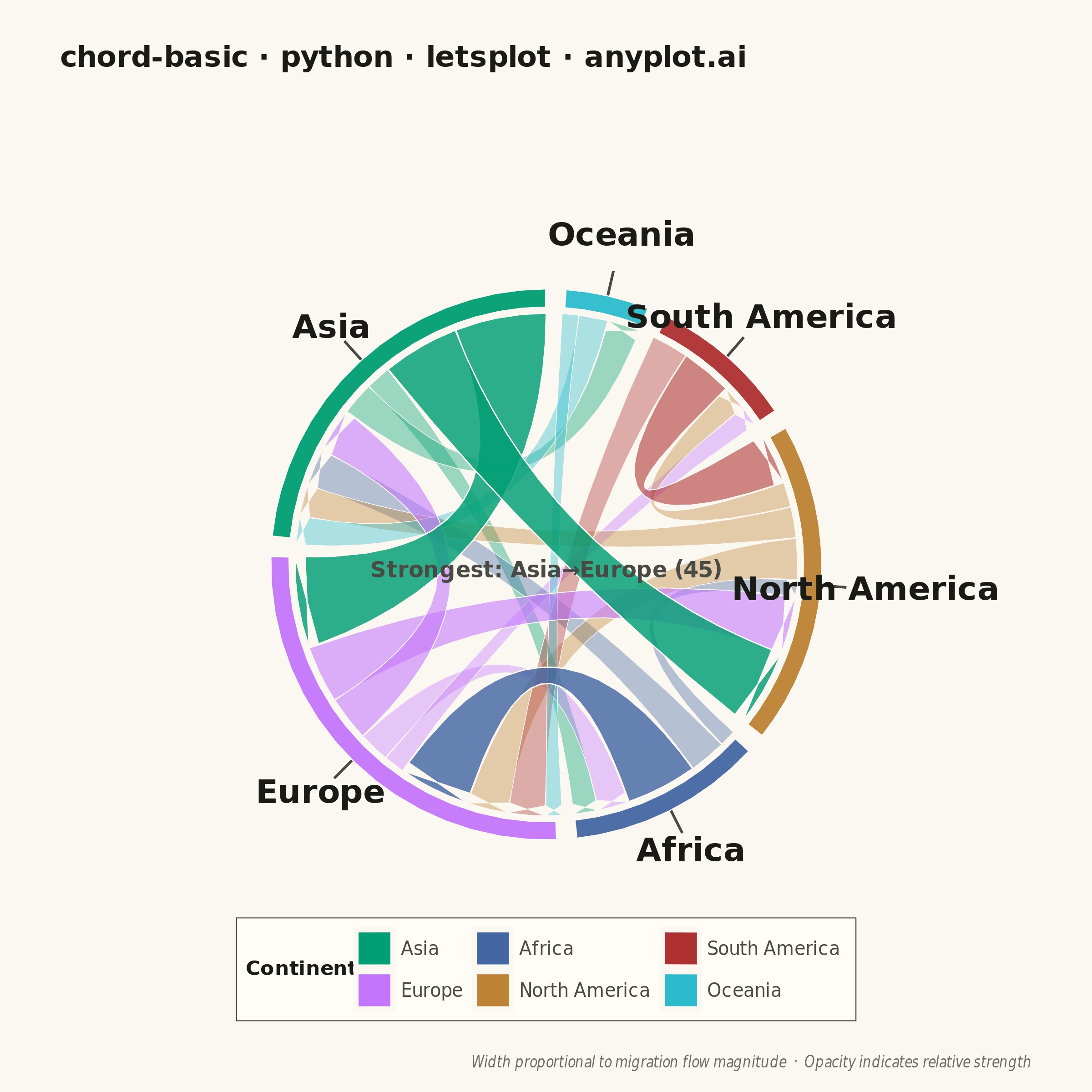
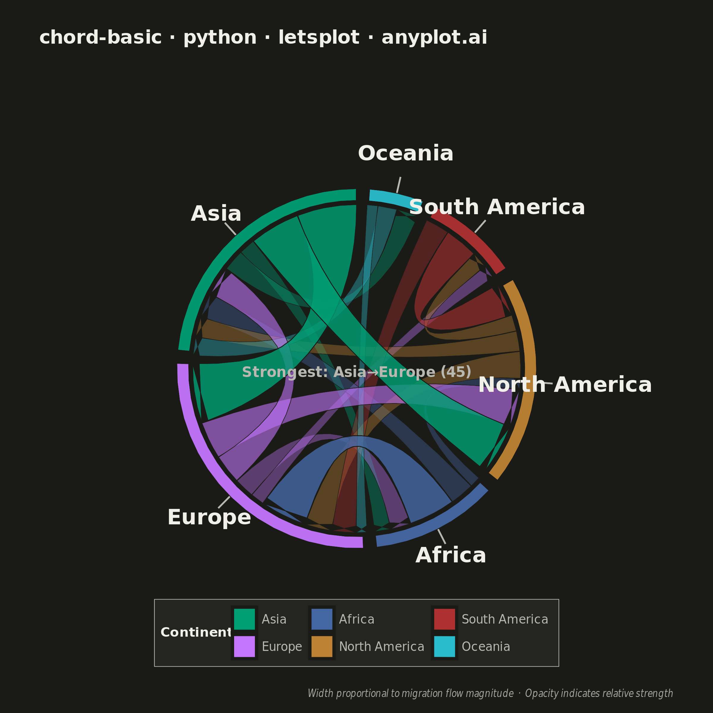
A chord diagram displays relationships or flows between entities arranged around a circle's perimeter. Arcs (chords) connect related entities, with chord width proportional to the flow magnitude. This visualization excels at revealing the overall structure of connections and identifying the strongest relationships within a system.
""" anyplot.ai
chord-basic: Basic Chord Diagram
Library: letsplot 4.10.1 | Python 3.13.14
Quality: 91/100 | Updated: 2026-06-17
"""

import math
import os

import numpy as np
import pandas as pd
from lets_plot import (
    LetsPlot,
    aes,
    coord_fixed,
    element_rect,
    element_text,
    geom_polygon,
    geom_segment,
    geom_text,
    ggplot,
    ggsize,
    labs,
    layer_tooltips,
    scale_fill_manual,
    scale_x_continuous,
    scale_y_continuous,
    theme,
    theme_void,
)
from lets_plot.export import ggsave
from PIL import Image


LetsPlot.setup_html()

# Theme-adaptive chrome (see prompts/default-style-guide.md "Theme-adaptive Chrome")
THEME = os.getenv("ANYPLOT_THEME", "light")
PAGE_BG = "#FAF8F1" if THEME == "light" else "#1A1A17"
ELEVATED_BG = "#FFFDF6" if THEME == "light" else "#242420"
INK = "#1A1A17" if THEME == "light" else "#F0EFE8"
INK_SOFT = "#4A4A44" if THEME == "light" else "#B8B7B0"
INK_MUTED = "#6B6A63" if THEME == "light" else "#A8A79F"
PAGE_BG_RGB = (250, 248, 241) if THEME == "light" else (26, 26, 23)

# Imprint palette — 8 hues, theme-independent, hybrid-v3 sort. First series ALWAYS #009E73.
IMPRINT_PALETTE = ["#009E73", "#C475FD", "#4467A3", "#BD8233", "#AE3030", "#2ABCCD", "#954477", "#99B314"]

# Migration flow data between continents (bidirectional flows)
flows = [
    ("Asia", "Europe", 45),
    ("Asia", "North America", 38),
    ("Asia", "Africa", 12),
    ("Asia", "Oceania", 16),
    ("Europe", "North America", 28),
    ("Europe", "Asia", 22),
    ("Europe", "Africa", 15),
    ("Europe", "South America", 10),
    ("Africa", "Europe", 35),
    ("Africa", "Asia", 18),
    ("Africa", "North America", 8),
    ("North America", "Europe", 20),
    ("North America", "Asia", 15),
    ("North America", "South America", 12),
    ("South America", "North America", 25),
    ("South America", "Europe", 18),
    ("Oceania", "Asia", 14),
    ("Oceania", "Europe", 8),
]

# Entities; first entity (Asia) gets Imprint brand green #009E73
entities = list(dict.fromkeys([f[0] for f in flows] + [f[1] for f in flows]))
colors = IMPRINT_PALETTE[: len(entities)]

# Calculate total flow for each entity (in + out)
entity_totals = dict.fromkeys(entities, 0)
for src, tgt, val in flows:
    entity_totals[src] += val
    entity_totals[tgt] += val

# Angular layout: proportional arc sizes with gaps
total_flow = sum(entity_totals.values())
gap_angle = 0.07
total_gap = gap_angle * len(entities)
available_angle = 2 * math.pi - total_gap

entity_arcs = {}
current_angle = math.pi / 2  # Start from top for better visual balance
for entity in entities:
    arc_size = (entity_totals[entity] / total_flow) * available_angle
    entity_arcs[entity] = {"start": current_angle, "end": current_angle + arc_size, "mid": current_angle + arc_size / 2}
    current_angle += arc_size + gap_angle

# Track offsets within each entity arc for chord placement
entity_offsets = {e: entity_arcs[e]["start"] for e in entities}

# Radius configuration
outer_radius = 1.0
inner_radius = 0.93
chord_radius = 0.91

# Build outer arc segments (the ring)
arc_data = []
n_arc_points = 80
for entity in entities:
    arc = entity_arcs[entity]
    angles = np.linspace(arc["start"], arc["end"], n_arc_points)
    for angle in angles:
        arc_data.append(
            {
                "x": outer_radius * np.cos(angle),
                "y": outer_radius * np.sin(angle),
                "entity": entity,
                "arc_id": f"{entity}_arc",
            }
        )
    for angle in reversed(angles):
        arc_data.append(
            {
                "x": inner_radius * np.cos(angle),
                "y": inner_radius * np.sin(angle),
                "entity": entity,
                "arc_id": f"{entity}_arc",
            }
        )

arc_df = pd.DataFrame(arc_data)

# Build chord polygons
flow_values = [f[2] for f in flows]
min_flow = min(flow_values)
max_flow = max(flow_values)

chord_data = []
chord_id = 0

for src, tgt, val in flows:
    src_width = (val / total_flow) * available_angle
    tgt_width = (val / total_flow) * available_angle

    src_start = entity_offsets[src]
    src_end = src_start + src_width
    entity_offsets[src] = src_end + 0.003

    tgt_start = entity_offsets[tgt]
    tgt_end = tgt_start + tgt_width
    entity_offsets[tgt] = tgt_end + 0.003

    n_bezier = 50
    src_angles = np.linspace(src_start, src_end, 12)
    tgt_angles = np.linspace(tgt_end, tgt_start, 12)

    polygon_x = []
    polygon_y = []

    # Source arc at chord_radius
    for angle in src_angles:
        polygon_x.append(chord_radius * np.cos(angle))
        polygon_y.append(chord_radius * np.sin(angle))

    # Bezier curve source → target (pulled toward circle center)
    src_end_x = chord_radius * np.cos(src_end)
    src_end_y = chord_radius * np.sin(src_end)
    tgt_start_x = chord_radius * np.cos(tgt_start)
    tgt_start_y = chord_radius * np.sin(tgt_start)

    for i in range(1, n_bezier):
        t = i / n_bezier
        x = (1 - t) ** 2 * src_end_x + 2 * (1 - t) * t * 0 + t**2 * tgt_start_x
        y = (1 - t) ** 2 * src_end_y + 2 * (1 - t) * t * 0 + t**2 * tgt_start_y
        polygon_x.append(x)
        polygon_y.append(y)

    # Target arc at chord_radius
    for angle in tgt_angles:
        polygon_x.append(chord_radius * np.cos(angle))
        polygon_y.append(chord_radius * np.sin(angle))

    # Bezier curve target → source
    tgt_end_x = chord_radius * np.cos(tgt_end)
    tgt_end_y = chord_radius * np.sin(tgt_end)
    src_start_x = chord_radius * np.cos(src_start)
    src_start_y = chord_radius * np.sin(src_start)

    for i in range(1, n_bezier):
        t = i / n_bezier
        x = (1 - t) ** 2 * tgt_end_x + 2 * (1 - t) * t * 0 + t**2 * src_start_x
        y = (1 - t) ** 2 * tgt_end_y + 2 * (1 - t) * t * 0 + t**2 * src_start_y
        polygon_x.append(x)
        polygon_y.append(y)

    for x, y in zip(polygon_x, polygon_y, strict=False):
        chord_data.append({"x": x, "y": y, "chord_id": f"chord_{chord_id}", "source": src, "target": tgt, "value": val})
    chord_id += 1

chord_df = pd.DataFrame(chord_data)

# Three-tier chord split for visual hierarchy (alpha floor raised so weak flows stay legible)
flow_threshold_high = min_flow + 0.66 * (max_flow - min_flow)
flow_threshold_mid = min_flow + 0.33 * (max_flow - min_flow)
chord_high = chord_df[chord_df["value"] >= flow_threshold_high]
chord_mid = chord_df[(chord_df["value"] >= flow_threshold_mid) & (chord_df["value"] < flow_threshold_high)]
chord_low = chord_df[chord_df["value"] < flow_threshold_mid]

# Entity labels with adaptive positioning to avoid crowding near small arcs
label_data = []
for entity in entities:
    arc = entity_arcs[entity]
    mid_angle = arc["mid"]
    arc_size = arc["end"] - arc["start"]
    label_radius = 1.16 + max(0, 0.12 * (1.0 - arc_size / 0.7))
    label_data.append({"x": label_radius * np.cos(mid_angle), "y": label_radius * np.sin(mid_angle), "label": entity})

label_df = pd.DataFrame(label_data)

# Tick marks connecting arcs to labels (visual refinement)
tick_data = []
for entity in entities:
    arc = entity_arcs[entity]
    mid_angle = arc["mid"]
    tick_data.append(
        {
            "x": outer_radius * np.cos(mid_angle),
            "y": outer_radius * np.sin(mid_angle),
            "xend": 1.09 * np.cos(mid_angle),
            "yend": 1.09 * np.sin(mid_angle),
        }
    )

tick_df = pd.DataFrame(tick_data)

# Annotation for dominant flow — data storytelling (positioned at center)
top_flow = max(flows, key=lambda f: f[2])
annotation_df = pd.DataFrame(
    [{"x": 0.0, "y": -0.02, "label": f"Strongest: {top_flow[0]}→{top_flow[1]} ({top_flow[2]})"}]
)

# Build the plot
plot = (
    ggplot()
    # Low-magnitude chords (background layer) — alpha raised from 0.2 for legibility
    + geom_polygon(
        aes(x="x", y="y", group="chord_id", fill="source"),
        data=chord_low,
        alpha=0.38,
        color=PAGE_BG,
        size=0.15,
        tooltips=layer_tooltips().line("@source → @target").line("Flow|@value"),
    )
    # Mid-magnitude chords
    + geom_polygon(
        aes(x="x", y="y", group="chord_id", fill="source"),
        data=chord_mid,
        alpha=0.58,
        color=PAGE_BG,
        size=0.2,
        tooltips=layer_tooltips().line("@source → @target").line("Flow|@value"),
    )
    # High-magnitude chords (foreground, most prominent)
    + geom_polygon(
        aes(x="x", y="y", group="chord_id", fill="source"),
        data=chord_high,
        alpha=0.82,
        color=PAGE_BG,
        size=0.25,
        tooltips=layer_tooltips().line("@source → @target").line("Flow|@value"),
    )
    # Outer arc segments (the entity ring)
    + geom_polygon(aes(x="x", y="y", group="arc_id", fill="entity"), data=arc_df, alpha=0.95, color=PAGE_BG, size=0.5)
    # Tick marks from arcs to labels
    + geom_segment(aes(x="x", y="y", xend="xend", yend="yend"), data=tick_df, color=INK_SOFT, size=0.6)
    # Entity labels
    + geom_text(aes(x="x", y="y", label="label"), data=label_df, size=9, color=INK, fontface="bold")
    # Dominant flow annotation for storytelling
    + geom_text(aes(x="x", y="y", label="label"), data=annotation_df, size=6, color=INK_SOFT, fontface="bold")
    # Scales and coordinates
    + scale_fill_manual(values=colors, name="Continent")
    + coord_fixed(ratio=1)
    + scale_x_continuous(limits=(-1.6, 1.6))
    + scale_y_continuous(limits=(-1.6, 1.6))
    + labs(
        title="chord-basic · python · letsplot · anyplot.ai",
        caption="Width proportional to migration flow magnitude  ·  Opacity indicates relative strength",
    )
    + ggsize(600, 600)
    + theme_void()
    + theme(
        plot_title=element_text(size=16, face="bold", color=INK),
        plot_caption=element_text(size=8, color=INK_MUTED, face="italic"),
        legend_text=element_text(size=10, color=INK_SOFT),
        legend_title=element_text(size=11, face="bold", color=INK),
        legend_position=[0.5, 0.03],
        legend_justification=[0.5, 0.0],
        legend_direction="horizontal",
        legend_background=element_rect(fill=ELEVATED_BG, color=INK_SOFT, size=0.5),
        panel_background=element_rect(fill=PAGE_BG, color=PAGE_BG, size=0),
        plot_background=element_rect(fill=PAGE_BG, color=PAGE_BG, size=0),
        plot_margin=[24, 16, 12, 16],
    )
)

# Save PNG (square: ggsize 600 × scale 4 = 2400×2400 px)
ggsave(plot, f"plot-{THEME}.png", path=".", scale=4)

# Flatten any residual transparency onto the theme page background
img = Image.open(f"plot-{THEME}.png").convert("RGBA")
bg = Image.new("RGBA", img.size, (*PAGE_BG_RGB, 255))
Image.alpha_composite(bg, img).convert("RGB").save(f"plot-{THEME}.png")

# Save interactive HTML export
ggsave(plot, f"plot-{THEME}.html", path=".")
Runnable source as JSON, for any HTTP client: https://api.anyplot.ai/specs/chord-basic/letsplot/code. Any spec id and library id listed in llms-full.txt fit the same URL shape; every URL below is complete and callable.
{
  "spec_id": "chord-basic",
  "language": "python",
  "library": "letsplot",
  "page": "https://anyplot.ai/chord-basic/python/letsplot",
  "hub": "https://anyplot.ai/chord-basic",
  "code_json": "https://api.anyplot.ai/specs/chord-basic/letsplot/code",
  "spec_json": "https://api.anyplot.ai/specs/chord-basic",
  "render_light_png": "https://storage.googleapis.com/anyplot-images/plots/chord-basic/python/letsplot/plot-light.png",
  "render_dark_png": "https://storage.googleapis.com/anyplot-images/plots/chord-basic/python/letsplot/plot-dark.png",
  "interactive_light_html": "https://storage.googleapis.com/anyplot-images/plots/chord-basic/python/letsplot/plot-light.html",
  "interactive_dark_html": "https://storage.googleapis.com/anyplot-images/plots/chord-basic/python/letsplot/plot-dark.html",
  "quality_score": 91.0,
  "license": "MIT",
  "guide": "https://anyplot.ai/llms.txt"
}
Part of Basic Chord Diagram on anyplot.ai.