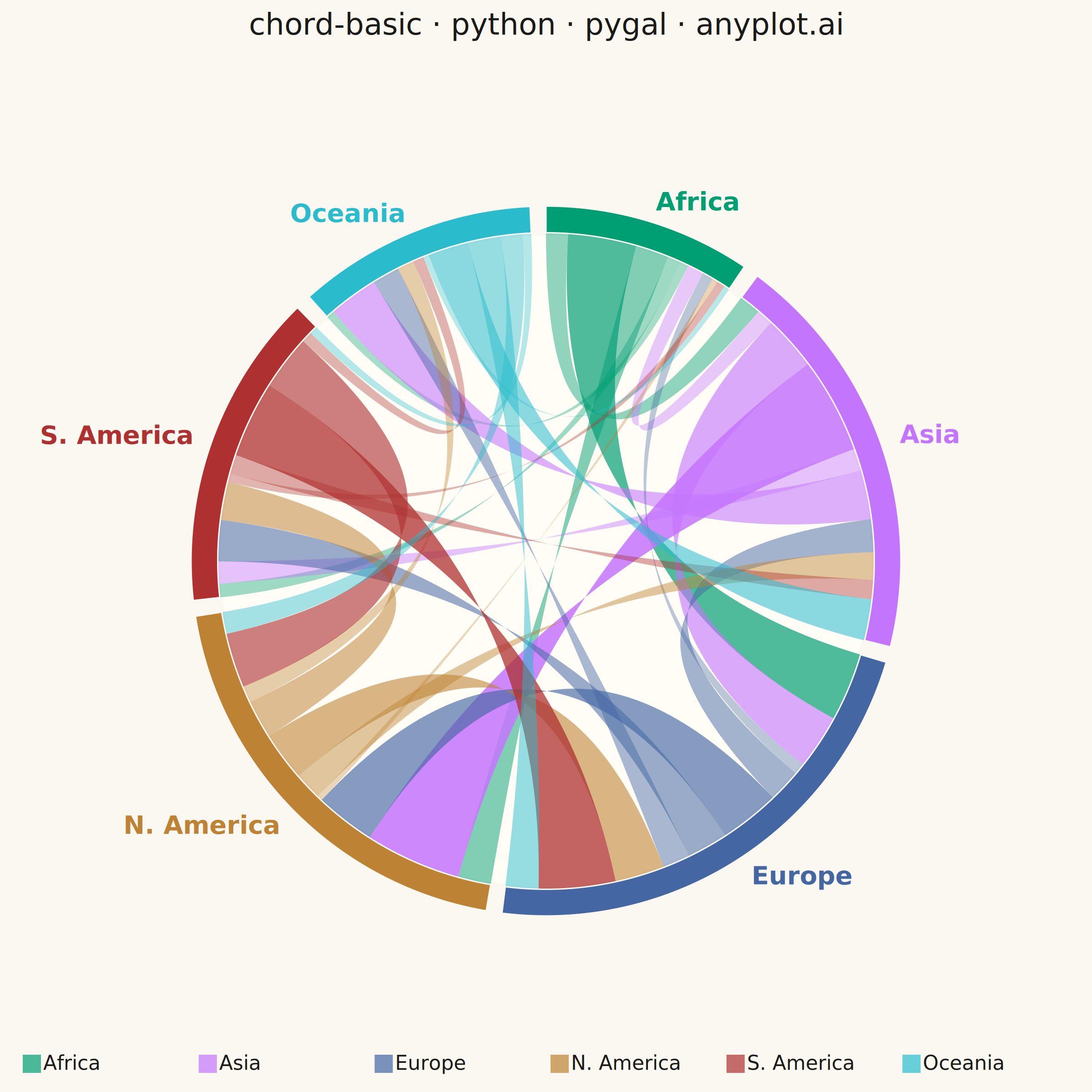
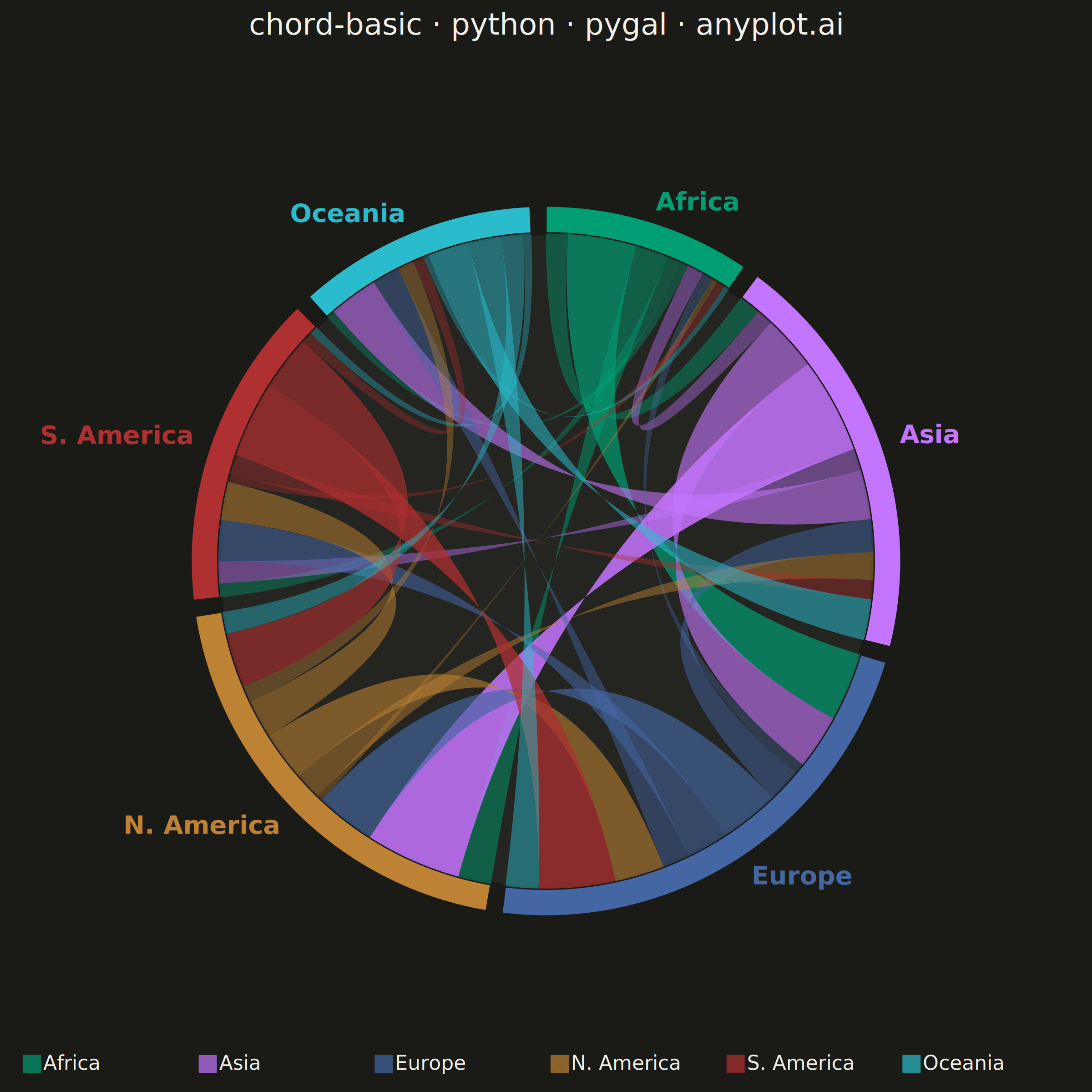
A chord diagram displays relationships or flows between entities arranged around a circle's perimeter. Arcs (chords) connect related entities, with chord width proportional to the flow magnitude. This visualization excels at revealing the overall structure of connections and identifying the strongest relationships within a system.
""" anyplot.ai
chord-basic: Basic Chord Diagram
Library: pygal 3.1.0 | Python 3.13.14
Quality: 93/100 | Updated: 2026-06-17
"""

import math
import os
import re

import cairosvg
import pygal
from pygal.style import Style


# Theme tokens (see prompts/default-style-guide.md "Theme-adaptive Chrome")
THEME = os.getenv("ANYPLOT_THEME", "light")
PAGE_BG = "#FAF8F1" if THEME == "light" else "#1A1A17"
ELEVATED_BG = "#FFFDF6" if THEME == "light" else "#242420"
INK = "#1A1A17" if THEME == "light" else "#F0EFE8"
INK_SOFT = "#4A4A44" if THEME == "light" else "#B8B7B0"
INK_MUTED = "#6B6A63" if THEME == "light" else "#A8A79F"

# Imprint palette — first series ALWAYS #009E73, then canonical order.
# Theme-independent so each continent keeps its identity across light/dark.
IMPRINT_PALETTE = (
    "#009E73",  # Africa     — brand green
    "#C475FD",  # Asia       — lavender
    "#4467A3",  # Europe     — blue
    "#BD8233",  # N. America — ochre
    "#AE3030",  # S. America — matte red
    "#2ABCCD",  # Oceania    — cyan
)

# Data: migration flows between 6 continents (thousands of people / year).
# Each (source, target, value) is one directed flow; both directions appear.
continents = ["Africa", "Asia", "Europe", "N. America", "S. America", "Oceania"]
n = len(continents)

flows = [
    (0, 1, 8),
    (0, 2, 25),
    (0, 3, 12),
    (0, 4, 5),
    (0, 5, 3),
    (1, 0, 6),
    (1, 2, 20),
    (1, 3, 35),
    (1, 4, 8),
    (1, 5, 18),
    (2, 0, 4),
    (2, 1, 12),
    (2, 3, 22),
    (2, 4, 15),
    (2, 5, 10),
    (3, 0, 2),
    (3, 1, 10),
    (3, 2, 18),
    (3, 4, 14),
    (3, 5, 6),
    (4, 0, 3),
    (4, 1, 7),
    (4, 2, 28),
    (4, 3, 20),
    (4, 5, 4),
    (5, 0, 2),
    (5, 1, 15),
    (5, 2, 12),
    (5, 3, 8),
    (5, 4, 3),
]

# Arc allocation proportional to total flow (in + out) per continent
totals = [0] * n
for s, t, v in flows:
    totals[s] += v
    totals[t] += v
grand_total = sum(totals)

# Square canvas — hard rule for symmetric circular plots (prompts/library/pygal.md)
W = H = 2400

# Style — pygal carries every theme token; sizes are native source pixels.
custom_style = Style(
    background=PAGE_BG,
    plot_background=PAGE_BG,
    foreground=INK,
    foreground_strong=INK,
    foreground_subtle=INK_MUTED,
    colors=IMPRINT_PALETTE,
    font_family="DejaVu Sans, Helvetica, Arial, sans-serif",
    title_font_family="DejaVu Sans, Helvetica, Arial, sans-serif",
    legend_font_family="DejaVu Sans, Helvetica, Arial, sans-serif",
    title_font_size=66,
    legend_font_size=44,
    stroke_width=0,
)

# Chart — pygal owns the title + bottom legend (one swatch per continent) and
# emits the interactive SVG/HTML. The chord geometry is injected afterwards in
# absolute pixel coordinates, so it never depends on pygal's internal padding.
chart = pygal.XY(
    width=W,
    height=H,
    style=custom_style,
    title="chord-basic · python · pygal · anyplot.ai",
    show_legend=True,
    legend_at_bottom=True,
    legend_at_bottom_columns=6,
    legend_box_size=40,
    show_x_labels=False,
    show_y_labels=False,
    show_x_guides=False,
    show_y_guides=False,
    stroke=False,
    dots_size=0,
    margin=40,
)

# One invisible anchor point per continent gives the legend its colored swatch
# without drawing anything in the plot area (and without a "No data" watermark).
for name in continents:
    chart.add(name, [(5, 5)], stroke=False, show_dots=False)

svg = chart.render().decode("utf-8")

# --- Locate title baseline + legend top so the diagram fits between them ---
title_ys = [float(y) for y in re.findall(r'<text x="[\d.]+" y="([\d.]+)" class="title"', svg)]
title_bottom = (max(title_ys) if title_ys else 80) + 70
m_leg = re.search(r'<g transform="translate\([\d.]+, ([\d.]+)\)" class="legends"', svg)
legend_top = float(m_leg.group(1)) if m_leg else H - 120

# Diagram geometry — all derived from canvas + parsed chrome, no magic numbers
cx = W / 2
cy = (title_bottom + legend_top) / 2
max_r_v = (legend_top - title_bottom) / 2 - 20
max_r_h = W / 2 - 340  # leave room for the widest side labels ("S. America")
r_label = min(max_r_v, max_r_h)
r_outer = r_label - 80  # colored band outer edge
band = r_outer * 0.075  # band thickness
r_inner = r_outer - band  # chords attach to the inner edge

# Arc spans (clockwise from top), proportional to each continent's total flow
gap = 0.045  # radians of whitespace between arcs
available = 2 * math.pi - gap * n
spans = [available * totals[i] / grand_total for i in range(n)]
arc_start = []  # higher angle (clockwise sweep decreases the angle)
angle = math.pi / 2  # start at the top
for i in range(n):
    arc_start.append(angle)
    angle -= spans[i] + gap

svg_elems = []

# Subtle hub disc to ground the circular composition
svg_elems.append(f'<circle cx="{cx:.1f}" cy="{cy:.1f}" r="{r_inner - 6:.1f}" fill="{ELEVATED_BG}" stroke="none"/>')

# Filled chord ribbons — width proportional to flow, colored by source,
# opacity scaled by magnitude so dominant corridors read first.
chord_r = r_inner
arc_pos = list(arc_start)
max_val = max(v for _, _, v in flows)
for s, t, v in flows:
    s_ext = spans[s] * v / totals[s]
    t_ext = spans[t] * v / totals[t]
    s_a1, s_a2 = arc_pos[s], arc_pos[s] - s_ext
    t_a1, t_a2 = arc_pos[t], arc_pos[t] - t_ext
    arc_pos[s] = s_a2
    arc_pos[t] = t_a2

    sx1, sy1 = cx + chord_r * math.cos(s_a1), cy - chord_r * math.sin(s_a1)
    sx2, sy2 = cx + chord_r * math.cos(s_a2), cy - chord_r * math.sin(s_a2)
    tx1, ty1 = cx + chord_r * math.cos(t_a1), cy - chord_r * math.sin(t_a1)
    tx2, ty2 = cx + chord_r * math.cos(t_a2), cy - chord_r * math.sin(t_a2)

    # Inset the quadratic control point toward — but short of — the hub: thick
    # corridors dive deep to the center, thin ones stay shallow, so the many
    # low-magnitude ribbons no longer pile up on a single point at the hub.
    depth = 0.55 + 0.35 * (v / max_val)
    c1x, c1y = (sx1 + tx1) / 2, (sy1 + ty1) / 2
    c2x, c2y = (tx2 + sx2) / 2, (ty2 + sy2) / 2
    q1x, q1y = c1x + depth * (cx - c1x), c1y + depth * (cy - c1y)
    q2x, q2y = c2x + depth * (cx - c2x), c2y + depth * (cy - c2y)

    opacity = 0.30 + 0.55 * (v / max_val)
    path = (
        f"M {sx1:.1f},{sy1:.1f} "
        f"Q {q1x:.1f},{q1y:.1f} {tx1:.1f},{ty1:.1f} "
        f"A {chord_r:.1f},{chord_r:.1f} 0 0,1 {tx2:.1f},{ty2:.1f} "
        f"Q {q2x:.1f},{q2y:.1f} {sx2:.1f},{sy2:.1f} "
        f"A {chord_r:.1f},{chord_r:.1f} 0 0,0 {sx1:.1f},{sy1:.1f} Z"
    )
    tip = f"{continents[s]} → {continents[t]}: {v}k/yr"
    svg_elems.append(
        f'<path d="{path}" fill="{IMPRINT_PALETTE[s]}" fill-opacity="{opacity:.2f}" '
        f'stroke="none"><title>{tip}</title></path>'
    )

# Node arcs — filled annular sectors on the perimeter, one per continent
for i in range(n):
    a0, a1 = arc_start[i], arc_start[i] - spans[i]
    ox1, oy1 = cx + r_outer * math.cos(a0), cy - r_outer * math.sin(a0)
    ox2, oy2 = cx + r_outer * math.cos(a1), cy - r_outer * math.sin(a1)
    ix2, iy2 = cx + r_inner * math.cos(a1), cy - r_inner * math.sin(a1)
    ix1, iy1 = cx + r_inner * math.cos(a0), cy - r_inner * math.sin(a0)
    sector = (
        f"M {ox1:.1f},{oy1:.1f} "
        f"A {r_outer:.1f},{r_outer:.1f} 0 0,1 {ox2:.1f},{oy2:.1f} "
        f"L {ix2:.1f},{iy2:.1f} "
        f"A {r_inner:.1f},{r_inner:.1f} 0 0,0 {ix1:.1f},{iy1:.1f} Z"
    )
    tip = f"{continents[i]}: {totals[i]}k/yr total flow"
    svg_elems.append(
        f'<path d="{sector}" fill="{IMPRINT_PALETTE[i]}" stroke="{PAGE_BG}" '
        f'stroke-width="3"><title>{tip}</title></path>'
    )

# Continent labels just outside their arc, colored for identity
for i, name in enumerate(continents):
    mid = arc_start[i] - spans[i] / 2
    lx, ly = cx + (r_outer + 46) * math.cos(mid), cy - (r_outer + 46) * math.sin(mid)
    deg = math.degrees(mid) % 360
    if deg <= 80 or deg >= 280:
        anchor = "start"
    elif 100 <= deg <= 260:
        anchor = "end"
    else:
        anchor = "middle"
    svg_elems.append(
        f'<text x="{lx:.1f}" y="{ly:.1f}" fill="{IMPRINT_PALETTE[i]}" '
        f'font-size="56" font-weight="bold" text-anchor="{anchor}" '
        f'dominant-baseline="central" '
        f'font-family="DejaVu Sans, Helvetica, Arial, sans-serif">{name}</text>'
    )

# Inject the diagram just before the closing tag and write outputs
svg = svg.replace("</svg>", "<g>" + "".join(svg_elems) + "</g></svg>")

with open(f"plot-{THEME}.svg", "w") as f:
    f.write(svg)

cairosvg.svg2png(bytestring=svg.encode("utf-8"), write_to=f"plot-{THEME}.png", output_width=W, output_height=H)

# Interactive HTML — embed the composed SVG so it matches the PNG exactly
with open(f"plot-{THEME}.html", "w") as f:
    f.write(
        '<!DOCTYPE html>\n<html>\n<head>\n<meta charset="utf-8">\n'
        "<title>chord-basic · python · pygal · anyplot.ai</title>\n"
        f"<style>body{{margin:0;background:{PAGE_BG}}}"
        "svg{width:100%;height:auto;display:block}</style>\n</head>\n<body>\n"
        f"{svg}\n</body>\n</html>"
    )
Runnable source as JSON, for any HTTP client: https://api.anyplot.ai/specs/chord-basic/pygal/code. Any spec id and library id listed in llms-full.txt fit the same URL shape; every URL below is complete and callable.
{
  "spec_id": "chord-basic",
  "language": "python",
  "library": "pygal",
  "page": "https://anyplot.ai/chord-basic/python/pygal",
  "hub": "https://anyplot.ai/chord-basic",
  "code_json": "https://api.anyplot.ai/specs/chord-basic/pygal/code",
  "spec_json": "https://api.anyplot.ai/specs/chord-basic",
  "render_light_png": "https://storage.googleapis.com/anyplot-images/plots/chord-basic/python/pygal/plot-light.png",
  "render_dark_png": "https://storage.googleapis.com/anyplot-images/plots/chord-basic/python/pygal/plot-dark.png",
  "interactive_light_html": "https://storage.googleapis.com/anyplot-images/plots/chord-basic/python/pygal/plot-light.html",
  "interactive_dark_html": "https://storage.googleapis.com/anyplot-images/plots/chord-basic/python/pygal/plot-dark.html",
  "quality_score": 93.0,
  "license": "MIT",
  "guide": "https://anyplot.ai/llms.txt"
}
Part of Basic Chord Diagram on anyplot.ai.