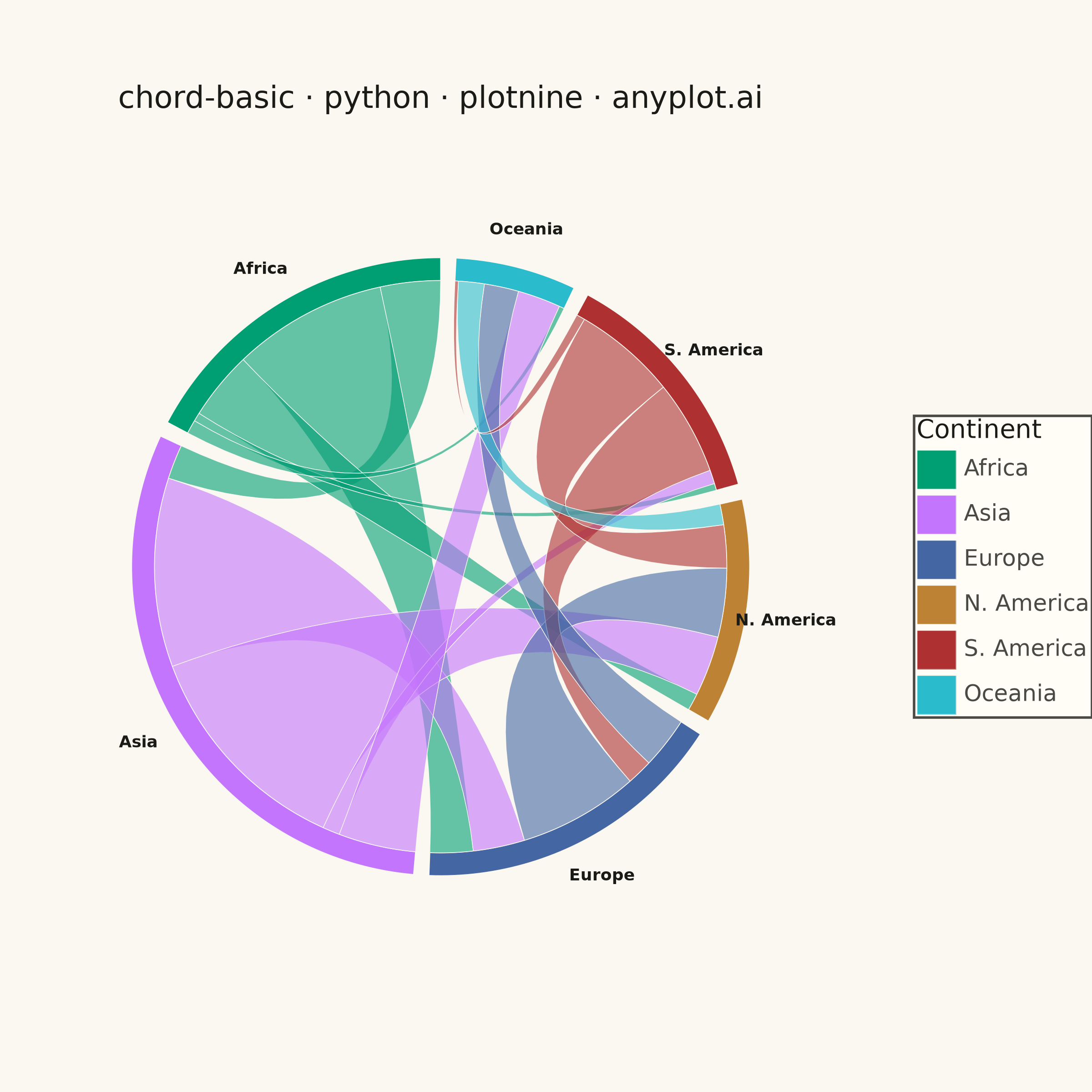
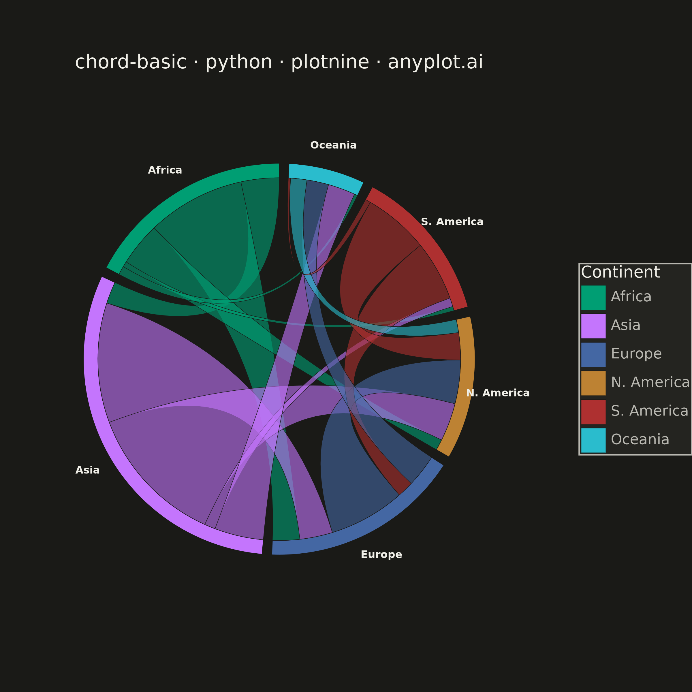
A chord diagram displays relationships or flows between entities arranged around a circle's perimeter. Arcs (chords) connect related entities, with chord width proportional to the flow magnitude. This visualization excels at revealing the overall structure of connections and identifying the strongest relationships within a system.
""" anyplot.ai
chord-basic: Basic Chord Diagram
Library: plotnine 0.15.7 | Python 3.13.13
Quality: 93/100 | Created: 2026-06-17
"""

import os

import numpy as np
import pandas as pd
from plotnine import (
    aes,
    coord_fixed,
    element_rect,
    element_text,
    geom_polygon,
    geom_text,
    ggplot,
    labs,
    scale_fill_manual,
    theme,
    theme_void,
)


# Theme tokens (see prompts/default-style-guide.md "Theme-adaptive Chrome")
THEME = os.getenv("ANYPLOT_THEME", "light")
PAGE_BG = "#FAF8F1" if THEME == "light" else "#1A1A17"
ELEVATED_BG = "#FFFDF6" if THEME == "light" else "#242420"
INK = "#1A1A17" if THEME == "light" else "#F0EFE8"
INK_SOFT = "#4A4A44" if THEME == "light" else "#B8B7B0"

# Imprint palette — abstract entities, canonical order, first series #009E73
IMPRINT_PALETTE = ["#009E73", "#C475FD", "#4467A3", "#BD8233", "#AE3030", "#2ABCCD"]

# Data — annual migration flows between 6 continents (thousands of people / year)
# Square directed matrix: M[i, j] = flow FROM entity i TO entity j (diagonal = 0)
continents = ["Africa", "Asia", "Europe", "N. America", "S. America", "Oceania"]
flow_matrix = np.array(
    [
        [0, 35, 90, 40, 5, 8],  # Africa -> ...
        [20, 0, 110, 130, 10, 45],  # Asia -> ...
        [25, 30, 0, 70, 15, 30],  # Europe -> ...
        [10, 35, 40, 0, 25, 12],  # N. America -> ...
        [4, 8, 55, 60, 0, 5],  # S. America -> ...
        [3, 25, 20, 15, 2, 0],  # Oceania -> ...
    ],
    dtype=float,
)
n = len(continents)

# Chord layout — each entity occupies an arc proportional to its total outflow,
# subdivided into one slice per destination (d3-style chord geometry)
group_value = flow_matrix.sum(axis=1)
total = group_value.sum()
pad = 0.05  # angular gap between adjacent entity arcs (radians)
scale = (2 * np.pi - n * pad) / total

sub_start = np.zeros((n, n))
sub_end = np.zeros((n, n))
group_a0 = np.zeros(n)
group_a1 = np.zeros(n)

angle = np.pi / 2  # start at the top of the circle
for i in range(n):
    group_a0[i] = angle
    cursor = angle
    for j in range(n):
        sub_start[i, j] = cursor
        cursor += flow_matrix[i, j] * scale
        sub_end[i, j] = cursor
    group_a1[i] = cursor
    angle = cursor + pad

# Radii: ribbons attach at R_IN; the entity arc band sits between R_IN and R_OUT
R_IN = 1.0
R_OUT = 1.08
R_LABEL = 1.22

# Outer entity arc bands (filled annular sectors)
arc_x, arc_y, arc_gid, arc_entity = [], [], [], []
for i in range(n):
    span = group_a1[i] - group_a0[i]
    steps = max(8, int(span / 0.02))
    outer = np.linspace(group_a0[i], group_a1[i], steps)
    inner = outer[::-1]
    xs = np.concatenate([R_OUT * np.cos(outer), R_IN * np.cos(inner)])
    ys = np.concatenate([R_OUT * np.sin(outer), R_IN * np.sin(inner)])
    arc_x.extend(xs)
    arc_y.extend(ys)
    arc_gid.extend([f"arc{i}"] * len(xs))
    arc_entity.extend([continents[i]] * len(xs))

arcs_df = pd.DataFrame({"x": arc_x, "y": arc_y, "gid": arc_gid, "entity": arc_entity})

# Ribbons — one per entity pair, ends curve through the circle centre.
# The dominant flow direction gives the ribbon its colour (its source entity).
rib_x, rib_y, rib_gid, rib_entity = [], [], [], []
t = np.linspace(0.0, 1.0, 28)  # quadratic Bezier parameter (control point = origin)
for i in range(n):
    for j in range(i + 1, n):
        if flow_matrix[i, j] == 0 and flow_matrix[j, i] == 0:
            continue
        src, dst = (i, j) if flow_matrix[i, j] >= flow_matrix[j, i] else (j, i)

        s0, s1 = sub_start[src, dst], sub_end[src, dst]
        d0, d1 = sub_start[dst, src], sub_end[dst, src]

        # source arc
        s_arc = np.linspace(s0, s1, 16)
        px = list(R_IN * np.cos(s_arc))
        py = list(R_IN * np.sin(s_arc))
        # Bezier from source end to destination start (curving through origin)
        x0, y0 = R_IN * np.cos(s1), R_IN * np.sin(s1)
        x1, y1 = R_IN * np.cos(d0), R_IN * np.sin(d0)
        px.extend((1 - t) ** 2 * x0 + t**2 * x1)
        py.extend((1 - t) ** 2 * y0 + t**2 * y1)
        # destination arc
        d_arc = np.linspace(d0, d1, 16)
        px.extend(R_IN * np.cos(d_arc))
        py.extend(R_IN * np.sin(d_arc))
        # Bezier back from destination end to source start
        x0, y0 = R_IN * np.cos(d1), R_IN * np.sin(d1)
        x1, y1 = R_IN * np.cos(s0), R_IN * np.sin(s0)
        px.extend((1 - t) ** 2 * x0 + t**2 * x1)
        py.extend((1 - t) ** 2 * y0 + t**2 * y1)

        rid = f"rib{src}_{dst}"
        rib_x.extend(px)
        rib_y.extend(py)
        rib_gid.extend([rid] * len(px))
        rib_entity.extend([continents[src]] * len(px))

ribbons_df = pd.DataFrame({"x": rib_x, "y": rib_y, "gid": rib_gid, "entity": rib_entity})

# Entity labels at the arc midpoints
mid = (group_a0 + group_a1) / 2
labels_df = pd.DataFrame({"x": R_LABEL * np.cos(mid), "y": R_LABEL * np.sin(mid), "entity": continents})

# Keep the legend / fill order stable
cat = pd.Categorical(continents, categories=continents, ordered=True)
arcs_df["entity"] = pd.Categorical(arcs_df["entity"], categories=continents)
ribbons_df["entity"] = pd.Categorical(ribbons_df["entity"], categories=continents)

# Plot
plot = (
    ggplot()
    + geom_polygon(arcs_df, aes(x="x", y="y", group="gid", fill="entity"), color=PAGE_BG, size=0.2)
    + geom_polygon(ribbons_df, aes(x="x", y="y", group="gid", fill="entity"), color=PAGE_BG, size=0.15, alpha=0.6)
    + geom_text(labels_df, aes(x="x", y="y", label="entity"), color=INK, size=6.5, fontweight="bold")
    + scale_fill_manual(values=IMPRINT_PALETTE, limits=list(cat.categories))
    + coord_fixed(ratio=1, xlim=(-1.4, 1.4), ylim=(-1.4, 1.4))
    + labs(title="chord-basic · python · plotnine · anyplot.ai", fill="Continent")
    + theme_void()
    + theme(
        figure_size=(6, 6),
        plot_background=element_rect(fill=PAGE_BG, color=PAGE_BG),
        panel_background=element_rect(fill=PAGE_BG, color=PAGE_BG),
        legend_background=element_rect(fill=ELEVATED_BG, color=INK_SOFT),
        legend_key=element_rect(fill=ELEVATED_BG, color=ELEVATED_BG),
        plot_title=element_text(size=12, color=INK, ha="center"),
        legend_title=element_text(size=10, color=INK),
        legend_text=element_text(size=9, color=INK_SOFT),
    )
)

# Save
plot.save(f"plot-{THEME}.png", dpi=400, width=6, height=6, units="in", verbose=False)
Runnable source as JSON, for any HTTP client: https://api.anyplot.ai/specs/chord-basic/plotnine/code. Any spec id and library id listed in llms-full.txt fit the same URL shape; every URL below is complete and callable.
{
  "spec_id": "chord-basic",
  "language": "python",
  "library": "plotnine",
  "page": "https://anyplot.ai/chord-basic/python/plotnine",
  "hub": "https://anyplot.ai/chord-basic",
  "code_json": "https://api.anyplot.ai/specs/chord-basic/plotnine/code",
  "spec_json": "https://api.anyplot.ai/specs/chord-basic",
  "render_light_png": "https://storage.googleapis.com/anyplot-images/plots/chord-basic/python/plotnine/plot-light.png",
  "render_dark_png": "https://storage.googleapis.com/anyplot-images/plots/chord-basic/python/plotnine/plot-dark.png",
  "quality_score": 93.0,
  "license": "MIT",
  "guide": "https://anyplot.ai/llms.txt"
}
Part of Basic Chord Diagram on anyplot.ai.